The modifiable areal unit problem (MAUP) is the fact that results from area-based data change when the areas change. It has two parts: the scale effect, from using bigger or smaller units, and the zoning effect, from drawing the boundaries differently. In Punjab, one correlation rose from 0.38 across 36 districts to 0.80 across 9 divisions. In Calgary, shifting a 2 km grid by less than a kilometre changed the share of residents counted in "high-density" cells from 8% to 18%.
Almost every map a client sees is built on someone else's boundaries: census tracts, postcodes, wards, districts, sales territories. Those lines were drawn for administration, not for your question, and the MAUP is the price of using them. This article shows how large that price can be with two real examples, and what to do about it.
What is the modifiable areal unit problem?
When data about people or events is grouped into areas, every number you compute from those areas, such as a rate, an average, a correlation or a hot spot, depends partly on how the areas were drawn. The units are "modifiable" because there is no single natural way to divide space. A different set of reasonable boundaries would give different results.
The term comes from Openshaw and Taylor's 1979 paper A Million or So Correlation Coefficients, and Openshaw's 1984 monograph The Modifiable Areal Unit Problem made it standard, though the effect was noticed as early as 1934, when Gehlke and Biehl found that correlations between census variables grew stronger as tracts were merged. Openshaw and Taylor regrouped Iowa's 99 counties into larger zones in many different ways and showed that the correlation between the share of residents over 65 and the Republican vote could be pushed from strongly negative to almost perfectly positive, using the same county data.
The MAUP has two parts:
| Effect | What changes | Example |
|---|---|---|
| Scale effect | The size and number of units | Districts vs divisions, tracts vs counties, H3 resolution 8 vs 6 |
| Zoning effect | Where boundaries fall, at roughly the same size | Two different ways to draw 9 regions, a grid shifted by half a cell |
Example 1: How does aggregation change a correlation in Punjab?
I used two district-level datasets behind this site's Punjab education map: girls' share of enrolment in government primary schools, from the Punjab Bureau of Statistics' 2022–23 education statistics, and the literacy rate of women aged 15 to 49, from MICS Punjab 2017–18. When districts are merged, both are averaged with primary enrolment as the weight.
The scale effect
| Variable pair | 36 districts | 9 divisions |
|---|---|---|
| Girls' share of primary enrolment vs women's literacy | 0.38 | 0.80 |
| College pupils per teacher vs women's literacy | −0.28 | −0.56 |
| Primary gender parity index vs women's literacy | 0.65 | 0.88 |
| Primary out-of-school rate vs women's literacy | −0.75 | −0.86 |
| Primary pupils per teacher vs out-of-school rate | 0.02 | 0.15 |
Every reasonably strong relationship got stronger when districts were grouped into divisions, and the weakest one more than doubled. That is the usual direction. Averaging cancels out district-level noise, so what remains is the broad north-south gradient that runs through most of Punjab's social indicators. The correlation at division level is not wrong. It answers a different question, about broad regions rather than districts, from only 9 data points.
The zoning effect
The official divisions are only one way to group 36 districts into 9. To see how much the boundaries themselves matter, I generated 1,000 random zonings: each one grows 9 contiguous regions from random seed districts across shared borders, so every region is a plausible block of neighbouring districts. I did the same for 18 and 4 regions.
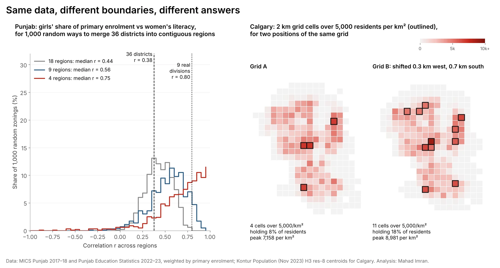
| Number of regions | Median r | Middle 90% of zonings | Full range |
|---|---|---|---|
| 36 (districts) | 0.38 | n/a | n/a |
| 18 | 0.44 | 0.19 to 0.66 | 0.00 to 0.79 |
| 9 | 0.56 | 0.16 to 0.81 | −0.32 to 0.93 |
| 4 | 0.75 | 0.16 to 0.98 | −0.87 to 1.00 |
Three things to notice:
- The median rises with aggregation. That is the scale effect again, now visible across many zonings rather than one.
- The spread widens fast. With 9 regions, the same underlying data supports a correlation anywhere from weakly negative to very strong. With 4 regions, almost any answer is available.
- The official divisions sit near the top. Only 6.9% of random 9-region zonings gave a correlation of 0.80 or more. Nobody drew Punjab's divisions to inflate this correlation, but a report that only used divisions would overstate the relationship compared with most other reasonable groupings.
Example 2: How does moving a grid change a density map?
Grids look neutral, which is why the zoning effect in them is easy to miss. I took Calgary's population on H3 resolution 8 hexagons from Kontur, assigned each hexagon's residents to the square grid cell containing its centre, and counted cells above 5,000 residents per km², a common threshold for "high density". Then I moved the grid's origin to 36 positions, in steps of a sixth of a cell, without changing its size.
| Cell size | Peak density across positions | Cells over 5,000/km² | Residents in those cells |
|---|---|---|---|
| 2 km | 6,770 to 11,168 per km² | 4 to 11 | 8% to 18% |
| 3 km | 4,980 to 8,059 per km² | 0 to 4 | 0% to 15% |
| 5 km | 3,429 to 5,028 per km² | 0 to 1 | 0% to 9% |
With a 2 km grid, a shift of 0.3 km west and 0.7 km south, about a third of a cell, took the high-density count from 4 cells holding 8% of residents to 11 cells holding 18%. The maps in the right half of the figure are the same city, same people and same cell size. A planner reading one would say Calgary has a handful of dense pockets. A planner reading the other would see a dense core and a ring of dense suburbs.
The scale effect runs alongside: the peak density at 5 km cells is roughly half of that at 2 km, because larger cells average dense blocks with roads, parks and industrial land. The same pattern drove the drop from 14,769 to 3,709 people per km² when the H3 resolution guide rolled Calgary up from resolution 8 to 6.
Where does the MAUP cause real problems?
- Site selection and trade areas. Population, income and competitor counts summed by postcode or tract can rank sites differently from the same data summed by drive-time polygon. That is one reason drive-time trade areas beat zone-based shortcuts.
- Hot spot maps. Getis-Ord Gi* and local Moran's I run on areas, so hot spots can appear, merge or vanish when the units change. The hot spot analysis walkthrough on Punjab's districts would produce a different map on tehsils.
- Choropleth maps. Large rural units dominate the visual impression while containing few people. Classification choices compound this, as shown in equal interval vs quantile vs natural breaks.
- Regression. Coefficients and R² shift with the units, as the correlations above did. A model fitted on districts says nothing reliable about tehsils or households. Geographically weighted regression on the same districts would also change if they were redrawn.
- Territories and electoral districts. Gerrymandering is the zoning effect used on purpose. Sales and franchise territories can be skewed the same way by accident, which is why franchise territory mapping should be balanced on households in small units.
How do you deal with the MAUP?
There is no statistical fix that removes it, because the dependence on units is real. The practical answer is to make results robust to it and honest about it.
- Start from the smallest units you can get. Individual records, geocoded points or the finest census geography give you room to aggregate deliberately later. Aggregating early throws the choice away.
- Match units to the question. If the decision is about a 10-minute drive, use drive-time areas. If it is about district funding, districts are the right unit, and the result should be stated as a district result.
- Run a sensitivity test. Rerun the analysis at two or three scales, and on at least one alternative zoning: a shifted grid, H3 hexagons, or randomly merged regions as above. If the conclusion survives, say so. If it does not, report the range.
- Use regular grids for comparison. H3 hexagons or a fixed square grid do not remove the zoning effect, but they make it testable and comparable between cities and years.
- Do not read area relationships as individual ones. A 0.80 correlation across divisions does not mean a literate mother is 80% likely to send a daughter to school. That inference is the ecological fallacy, and the MAUP makes it worse.
- Watch the small numbers. Rates in units with few people are noisy, and some extreme values on a choropleth are just small denominators. Smoothing or minimum-population thresholds help.
A sensitivity test needs very little code. With GeoPandas, a random contiguous regrouping can be built by growing regions from random seeds across a contiguity graph, as I did here, and a grid shift is two lines:
import numpy as np

def grid_cells(x, y, size, ox=0.0, oy=0.0):
    """Assign projected points to square cells of `size` metres, offset by (ox, oy)."""
    return np.floor((x - ox) / size).astype(int), np.floor((y - oy) / size).astype(int)

# Rerun the same summary for many offsets and report the range
for ox in np.linspace(0, 2000, 6, endpoint=False):
    for oy in np.linspace(0, 2000, 6, endpoint=False):
        ix, iy = grid_cells(x, y, 2000, ox, oy)
        # ... aggregate, then compute peak density, cells above threshold, etc.
What are the limits of these examples?
- The Punjab variables come from two sources and years. Enrolment shares are from 2022–23 and literacy from MICS 2017–18. The point here is how the correlation moves with the units, not its exact value.
- Weights matter. I weighted district values by primary enrolment when merging. Population weights would give somewhat different numbers, though the pattern of widening ranges would remain.
- The Calgary grid uses hexagon centres. Residents are assigned to cells by the centre of their resolution 8 hexagon, about 0.74 km², so 2 km cells are near the smallest size this data supports.
What should you take from this?
Any result from area data carries the boundaries it was computed on. Before presenting a correlation, a hot spot or a density ranking, rerun it on a second set of units. If it holds, you have a stronger finding to show a client. If it moves a lot, that movement is itself the finding, and it is far better to discover it before the decision than after.
If you need an analysis that has to hold up to scrutiny, from site rankings to district targeting, email me at mahad.imran29@gmail.com.