Hot spot analysis tests whether high or low values cluster in space more than chance would allow. On female literacy across Punjab's 36 districts, global Moran's I was 0.58, and none of 9,999 random reshuffles of the same values came close (the highest was 0.42). Getis-Ord Gi then found 8 hot-spot districts in the north-east and 7 cold-spot districts in the south-west, and 12 of those 15 survived a false discovery rate correction.*
This article explains the three statistics most people mean by "hot spot analysis" (global Moran's I, local Moran's I and Getis-Ord Gi*), runs all three on one real dataset, and shows where they agree, where they disagree and why. It ends with Python code and the matching tools in ArcGIS Pro and GeoDa.
What is hot spot analysis?
Hot spot analysis is a family of spatial statistics that ask one question: do the high values (or the low values) of a variable sit next to each other more than random placement would produce? A choropleth shows a pattern. A hot spot statistic tells you whether it is stronger than what random shuffling of the same values would draw.
Three statistics do most of the work:
| Global Moran's I | Local Moran's I (LISA) | Getis-Ord Gi* | |
|---|---|---|---|
| Question | Is there clustering anywhere on the map? | Where are the clusters, and are there outliers? | Where are the concentrations of high and low values? |
| Output | One number and one p-value | One value per area, plus a cluster type | One z-score per area |
| Finds spatial outliers? | No | Yes (High-Low, Low-High) | No |
| ArcGIS Pro tool | Spatial Autocorrelation (Global Moran's I) | Cluster and Outlier Analysis (Anselin Local Moran's I) | Hot Spot Analysis (Getis-Ord Gi*) |
| PySAL class | esda.Moran | esda.Moran_Local | esda.G_Local(star=True) |
| Source | Moran, 1950 | Anselin, 1995 | Ord and Getis, 1995 |
The usual workflow is global first, then local. If global Moran's I shows no clustering, local hot spots are more likely to be noise.
What data did I use?
The indicator is the literacy rate of women aged 15 to 49, by district, from the Multiple Indicator Cluster Survey (MICS) Punjab 2017-18, run by the Bureau of Statistics Punjab with UNICEF. It is one of the layers on this site's Punjab education map.
Values run from 26.1% in Rajanpur to 78.3% in Gujrat, with a mean of 54.0%. In the choropleth classification comparison I noted that this indicator is spread fairly evenly, with no long tail, which makes it a clean test case: any clustering found here comes from where the values sit.
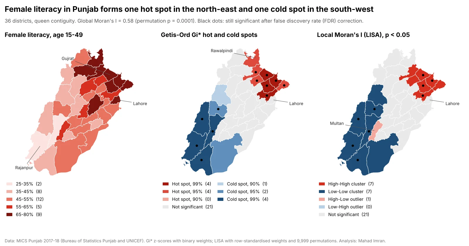
Same 36 districts, same queen contiguity. Black dots mark districts that remain significant after the false discovery rate correction. Legend counts are numbers of districts.
How do you choose spatial weights?
Every statistic here depends on a spatial weights matrix, which defines who counts as a neighbour. It is the most important choice in the analysis, and it should be made before looking at results.
The common options:
- Queen contiguity: areas sharing an edge or a corner are neighbours. A sensible default for administrative polygons.
- Rook contiguity: only shared edges count.
- K nearest neighbours: each area gets exactly k neighbours by centroid distance. Useful when neighbour counts vary wildly.
- Distance band: everything within a fixed distance. The ArcGIS Pro default for Hot Spot Analysis, and a good fit for points or equal-sized cells.
I used queen contiguity. On these boundaries it gives exactly the same neighbours as rook (no districts touch only at a corner), with a mean of 4.8 neighbours per district and a range from 2 (Narowal) to 9 (Jhang). Border districts such as Narowal and Lahore lose neighbours on the Indian side and across provincial lines. That edge effect is real and worth stating in any report.
Two more decisions:
- Row-standardise for Moran's I. Each district's weights are divided by its number of neighbours, so the "spatial lag" becomes the neighbours' average and well-connected districts do not dominate.
- Use binary weights for Gi.* Gi* sums the values in a neighbourhood that includes the district itself. I used plain 1/0 weights, the standard form of the statistic.
A sensitivity check takes a minute: global Moran's I was 0.58 with queen weights, 0.59 with 4 nearest neighbours and 0.49 with 6.
If your data are points (crimes, crashes, customer addresses), aggregate them to equal-sized cells first. Hexagons make neighbour definitions uniform, and the H3 resolution guide covers how to pick a cell size.
What is global Moran's I and how do you read it?
Global Moran's I measures how similar each area's value is to the average of its neighbours, across the whole map. It runs roughly from -1 (neighbours systematically unlike each other, as on a chessboard) through about 0 (no pattern) to +1 (neighbours very alike). Under no spatial pattern its expected value is -1/(n-1), which for 36 districts is -0.029.
With row-standardised weights:
I = Σ zi · lagi / Σ zi²
where zi is each district's deviation from the mean and lagi is the average deviation of its neighbours.
For Punjab female literacy, I = 0.581.
To test it, I used a permutation test. The 36 values were shuffled randomly across the 36 districts 9,999 times and Moran's I recomputed each time. The highest shuffled value was 0.424, and none reached 0.581, so the pseudo p-value is 1/(9,999+1) = 0.0001, the smallest this number of permutations can give. The analytical z-score was 5.93, which agrees.
For comparison, the primary out-of-school rate scored 0.64 and the primary gender parity index 0.42. Global Moran's I says clustering exists. Locating it is the job of the local statistics.
How does Getis-Ord Gi* find hot spots?
Getis-Ord Gi* takes each district, adds up its own value and its neighbours' values, and compares that local sum with what the sum would be if the neighbourhood were average. The result is a z-score. A large positive z-score means a neighbourhood of high values (a hot spot). A large negative one means a neighbourhood of low values (a cold spot).
The standard reporting, used by ArcGIS Pro's Hot Spot Analysis (Getis-Ord Gi*) tool in its Gi_Bin field, sorts the z-scores into confidence bins:
| Gi_Bin | Meaning | Absolute z-score at least | Punjab districts |
|---|---|---|---|
| 3 | Hot spot, 99% confidence | 2.58 | 4 |
| 2 | Hot spot, 95% confidence | 1.96 | 4 |
| 1 | Hot spot, 90% confidence | 1.65 | 0 |
| 0 | Not significant | 21 | |
| -1 | Cold spot, 90% confidence | 1.65 | 1 |
| -2 | Cold spot, 95% confidence | 1.96 | 2 |
| -3 | Cold spot, 99% confidence | 2.58 | 4 |
The 99% hot spots are Sialkot (z = 3.27), Gujrat (3.20), Sheikhupura (2.78) and Gujranwala (2.63). The 99% cold spots are Rajanpur (-3.01), Muzaffargarh (-2.94), Dera Ghazi Khan (-2.84) and Rahim Yar Khan (-2.59).
Two results show what Gi* measures:
- Sheikhupura is a 99% hot spot with literacy of 63.1%, only 9 points above the provincial mean. Its six neighbours include Sialkot, Lahore, Gujranwala and Narowal, all above 72%. Gi* scores the neighbourhood, so a middling district surrounded by high ones can be a strong hot spot.
- Lahore, at 75.3% the fourth-highest district, is not a hot spot (z = 1.01). Its three neighbours, Kasur, Nankana Sahib and Sheikhupura, average 55.9%. One high value on its own does not make a concentration.
How is local Moran's I (LISA) different?
Local Moran's I gives each district a score for how similar it is to its neighbours, and then a cluster type based on whether the district and its neighbourhood are above or below the mean:
- High-High: high value, high neighbours. A cluster of high values.
- Low-Low: low value, low neighbours.
- High-Low: high value, low neighbours. A spatial outlier.
- Low-High: low value, high neighbours. Also an outlier.
Significance comes from conditional permutation: each district's value is held fixed while its neighbours are drawn at random from the other districts, 9,999 times.
At p < 0.05, LISA found 7 High-High districts (Sialkot, Gujrat, Gujranwala, Sheikhupura, Jhelum, Mandi Bahauddin and Narowal), 7 Low-Low districts (Rajanpur, Muzaffargarh, Dera Ghazi Khan, Rahim Yar Khan, Layyah, Bahawalpur and Bhakkar) and 1 High-Low outlier: Multan.
Multan's female literacy is 57.1%, above the provincial mean, while its four neighbours (Bahawalpur, Muzaffargarh, Khanewal and Lodhran) average 42.4%. It is an urban centre inside the southern cold spot. Gi* gives Multan a z-score of -1.48, not significant, because its low neighbours outweigh its own value in the local sum. Only LISA can see it.
Gi* hot spot or LISA High-High: which should you report?
Use Gi* when the question is "where are values concentrated?" and LISA when you also need to know which areas break the local pattern. On this dataset they agree on the core and differ at the edges:
| District | Literacy | Gi* z-score | Gi* result | LISA result | Why they differ |
|---|---|---|---|---|---|
| Sialkot | 78.1% | 3.27 | Hot, 99% | High-High | Agree |
| Sheikhupura | 63.1% | 2.78 | Hot, 99% | High-High | Agree |
| Rawalpindi | 77.2% | 2.09 | Hot, 95% | Not significant (p = 0.07) | Gi* counts its own high value. Neighbour Attock (51.8%) weakens the LISA test |
| Narowal | 73.8% | 2.26 | Hot, 95% | High-High (p = 0.0497) | Borderline: significant in 13 of 20 random seeds |
| Lahore | 75.3% | 1.01 | Not significant | Not significant | Agree: high value, ordinary neighbours |
| Multan | 57.1% | -1.48 | Not significant | High-Low outlier | Gi* cannot express an outlier |
| Bhakkar | 41.0% | -1.89 | Cold, 90% | Low-Low (p = 0.048) | Borderline: significant in 17 of 20 LISA seeds |
| Rajanpur | 26.1% | -3.01 | Cold, 99% | Low-Low | Agree |
The general differences:
- Gi includes the area itself; LISA compares the area with its neighbours.* A very high district with mixed neighbours can be a Gi* hot spot and not a LISA cluster (Rawalpindi), and a middling district inside a high neighbourhood can be a strong Gi* hot spot (Sheikhupura).
- Gi has no outlier category.* If outliers matter (a well-served town inside an underserved region), use LISA.
- Gi is easier to explain.* "A cluster of high values, 99% confidence" reads well in a report.
My default for a client report is Gi* as the headline map, with LISA run alongside to catch outliers.
Why does the small number of districts matter?
With 36 areas, every statistic here has little information to work with. Esri recommends at least 30 features for Hot Spot Analysis, and Punjab only just clears that line. Three practical consequences:
- Borderline districts are unstable. I reran LISA with 20 different random seeds. Narowal's p-value ranged from 0.045 to 0.053, and Bhakkar's from 0.045 to 0.050. Report districts near p = 0.05 as uncertain, and fix the random seed so your numbers can be reproduced.
- Use enough permutations. ArcGIS Pro's Cluster and Outlier Analysis defaults to 499 permutations, which cannot produce a p-value below 0.002. For a final result use 9,999.
- Each value is itself an estimate. MICS district figures come from a household sample, so small gaps between neighbours may be sampling error.
What is the false discovery rate correction and should you use it?
Each district is a separate significance test. At 95% confidence, about 1 test in 20 comes out significant by chance even with no pattern, and neighbouring tests share data. A false discovery rate (FDR) correction lowers the p-value threshold to control the expected share of false positives among the significant results. ArcGIS Pro offers it as the "Apply False Discovery Rate (FDR) Correction" option, and GeoDa offers it alongside Bonferroni bounds in the significance filter.
On Punjab female literacy, using the Benjamini-Hochberg procedure in PySAL's esda.fdr:
| Uncorrected | With FDR | |
|---|---|---|
| Gi* significant districts (90% or higher) | 15 | 12 |
| Gi* districts at 99% | 8 | 0 |
| LISA High-High | 7 | 4 |
| LISA Low-Low | 7 | 5 |
| LISA High-Low (Multan) | 1 | 0 |
The FDR threshold at 95% was p ≤ 0.0125, and at 99% no district qualified at all. What survives is the same core on both methods: Sialkot, Gujrat, Gujranwala and Sheikhupura in the north-east, and Rajanpur, Muzaffargarh, Dera Ghazi Khan, Rahim Yar Khan and Layyah in the south-west. Those are the districts I would name with confidence. The others stay on the map as weaker evidence.
How do you do hot spot analysis in Python?
PySAL covers all three statistics, through the libpysal package for weights and esda for the statistics. This is the code behind every number above (libpysal 4.15, esda 2.10):
import numpy as np
import geopandas as gpd
from libpysal.weights import Queen
from esda import Moran, Moran_Local, G_Local, fdr

gdf = gpd.read_file("punjab_districts.gpkg")
y = gdf["female_lit"].to_numpy()

# Queen contiguity: districts sharing an edge or a corner are neighbours
w = Queen.from_dataframe(gdf, use_index=False)
w.transform = "r"                       # row-standardise for Moran's I

np.random.seed(12345)                   # permutation results vary slightly by seed
mi = Moran(y, w, permutations=9999)
print(f"Moran's I = {mi.I:.3f}, pseudo p = {mi.p_sim:.4f}")

# Local Moran's I (LISA): quadrant 1=HH, 2=LH, 3=LL, 4=HL
np.random.seed(12345)
lisa = Moran_Local(y, w, permutations=9999)
labels = np.array(["", "HH", "LH", "LL", "HL"])[lisa.q]
gdf["lisa"] = np.where(lisa.p_sim < 0.05, labels, "ns")
gdf["lisa_fdr"] = np.where(lisa.p_sim <= fdr(lisa.p_sim, 0.05), labels, "ns")

# Getis-Ord Gi*: binary weights, focal district included (star=True)
w.transform = "b"
gi = G_Local(y, w, transform="B", star=True, permutations=9999)
gdf["gi_z"] = gi.Zs                     # analytical z-score, as in ArcGIS Pro
gdf["gi_bin"] = np.sign(gi.Zs) * np.digitize(np.abs(gi.Zs), [1.645, 1.96, 2.576])
I checked the Gi* z-scores against a direct NumPy implementation of the Ord and Getis formula and they matched to 15 decimal places.
In ArcGIS Pro, use Spatial Autocorrelation (Global Moran's I), Hot Spot Analysis (Getis-Ord Gi*) and Cluster and Outlier Analysis (Anselin Local Moran's I) in the Spatial Statistics toolbox. For polygons, set Conceptualization of Spatial Relationships to contiguity edges and corners, tick the FDR option and raise the permutations. Optimized Hot Spot Analysis chooses a distance band and applies FDR for you, which also hides the weights decision.
In GeoDa, create queen contiguity weights in the Weights Manager, then run Space, Univariate Local Moran's I for the LISA cluster map and Local G* for hot spots. The GeoDa local autocorrelation workbook walks through the significance filter, including the FDR and Bonferroni options.
What should you take from this?
Run global Moran's I first to confirm there is clustering at all. Then map Gi* for hot and cold spots and LISA for outliers, using weights you chose before seeing the results. Apply the FDR correction, name only the areas that survive it with confidence, and treat anything near p = 0.05 as provisional, especially with fewer than about 50 areas. On Punjab's female literacy that leaves a clear, defensible story: a strong north-eastern cluster around Sialkot, Gujrat and Gujranwala, a strong south-western one around Rajanpur and Dera Ghazi Khan, and Multan standing apart from its region.
If you need hot spot analysis run on your own district, incident or customer data, with the weights and significance choices documented for review, email me at mahad.imran29@gmail.com.