A choropleth map shades areas by class, and the classification method decides where the class boundaries fall. I mapped the share of primary-age children out of school in Punjab's 36 districts three ways. Equal interval and natural breaks each put 2 districts in the darkest class. Quantile put 7 there, including one with half the rate of the worst.
This article walks through the three common methods on that one dataset, shows where each misleads, and gives a short rule for choosing, plus the related decisions that matter as much: the number of classes, rates versus counts, and legends.
What is choropleth classification?
A choropleth map colours each area, such as a district, county or census tract, according to a value. Unless you use a continuous colour ramp, the values are first grouped into a small number of classes, and each class gets one colour.
The classification method is the rule that draws the class boundaries. Change the rule and the same district can move from pale to dark without its value changing. Readers see the colours, not the numbers, so the method is part of the message.
The three methods most people meet first:
| Method | How it draws boundaries | Class sizes |
|---|---|---|
| Equal interval | Splits the range from minimum to maximum into equal-width steps | Vary, often very uneven on skewed data |
| Quantile | Puts the same number of areas in each class | Equal by construction |
| Natural breaks (Jenks) | Places boundaries at the largest gaps in the sorted values, minimising variance within classes | Vary with the data |
Natural breaks is the default for graduated colours in ArcGIS Pro, with five classes, according to the ArcGIS Pro SDK reference. That default is why so many published maps use it without anyone having chosen it.
What happens when one dataset is mapped three ways?
The data are from the Multiple Indicator Cluster Survey (MICS) Punjab 2017-18, run by the Bureau of Statistics Punjab with UNICEF. The indicator is the percentage of primary-school-age children who are out of school, for each of Punjab's 36 districts. It is one of the layers on this site's Punjab education map.
The values run from 3.1% in Narowal to 33.4% in Rajanpur. The median district is 10.4% and the mean 12.5%, because a handful of southern districts pull the average up. Most districts sit between 5% and 15%, with a long tail.
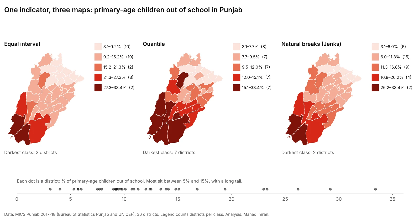
Same data, five classes each. Legend counts are the number of districts in each class.
| Class | Equal interval | Quantile | Natural breaks |
|---|---|---|---|
| 1 (lightest) | 3.1–9.2% (10) | 3.1–7.7% (8) | 3.1–6.0% (6) |
| 2 | 9.2–15.2% (19) | 7.7–9.5% (7) | 6.0–11.3% (15) |
| 3 | 15.2–21.3% (2) | 9.5–12.0% (7) | 11.3–16.8% (9) |
| 4 | 21.3–27.3% (3) | 12.0–15.1% (7) | 16.8–26.2% (4) |
| 5 (darkest) | 27.3–33.4% (2) | 15.1–33.4% (7) | 26.2–33.4% (2) |
Equal interval: honest scale, little detail
Equal interval treats every 6 percentage points the same, which is easy to explain. But 19 of the 36 districts land in one class, from 9.2% to 15.2%. On the map, most of central and eastern Punjab is a single colour, even though that class includes both Lahore (9.2%) and Multan (14.8%), whose rates differ by more than half.
This is the general weakness of equal interval: with skewed data, the outliers set the class width and the bulk of the areas are squeezed into one or two classes.
Quantile: every colour used, but the top class stretches
Quantile gives each class seven or eight districts, so the map uses its whole colour range and shows a clear ranking. It is the map that looks most "informative".
The cost is in the darkest class, which runs from 15.1% to 33.4%. Khushab, at 16.8%, is shaded the same as Rajanpur at 33.4%. A reader would assume they share a problem of the same size. Meanwhile the three middle classes are each less than 3 points wide, so Okara (10.7%) and Khanewal (12.5%) are separated by a colour step for a difference smaller than many survey margins of error.
Quantile maps answer "which districts are in the worst fifth?" well. They answer "how bad is it?" badly.
Natural breaks: follows the data, hard to compare
Natural breaks put the boundaries in the gaps: between Sialkot (6.0%) and Sargodha (7.5%), between Khushab (16.8%) and Muzaffargarh (19.4%), and between Bahawalpur (26.2%) and Rahim Yar Khan (29.2%). The two worst districts, Rahim Yar Khan and Rajanpur, stand alone in the darkest class, and the south-western cluster is clearly separated from the rest.
A standard measure of how well classes fit the data, the goodness of absolute deviation fit (GADF, where 1 is a perfect fit), confirms it: natural breaks scored 0.78, quantile 0.71 and equal interval 0.67 on this dataset, computed with the Python library mapclassify.
The weakness is that the breaks are odd numbers that come from this dataset only. Map the 2023 survey with natural breaks and the boundaries will move, so two maps that look alike may mean different things. That makes natural breaks a poor choice for a series of maps meant to be compared.
Does this depend on the indicator?
Yes, and that is the point. I ran the same three methods on two more Punjab indicators:
| Indicator | Equal interval, darkest class | Quantile, darkest class | Natural breaks, darkest class |
|---|---|---|---|
| Primary-age children out of school (%) | 2 districts | 7 districts | 2 districts |
| Pupils per teacher, government primary schools | 3 districts | 7 districts | 2 districts |
| Literacy rate, women aged 15–49 (%) | 8 districts | 7 districts | 7 districts |
Female literacy is spread fairly evenly from 26% to 78%, with no long tail, so all three methods agree on the seven or eight best-performing districts in the north and north-east. The other two indicators are skewed, and the methods disagree. The more skewed the data, the more the method matters. Check the distribution before choosing, which takes one histogram or dot plot.
How should you choose a classification method?
Choose based on the question the map must answer, and choose before looking at the results.
| If the map needs to... | Use | Why |
|---|---|---|
| Rank areas for a general audience | Quantile | Equal-sized classes read naturally as "top fifth, bottom fifth". In Brewer and Pickle's 2002 study of mortality maps, quantile and minimum-boundary-error methods were the most accurate for general map-reading tasks. |
| Show real clusters in skewed data | Natural breaks | Keeps similar values together and isolates genuine outliers. |
| Compare maps across years or regions | Fixed breaks shared by all maps | Brewer and Pickle found matched legends across a series improved map-comparison accuracy by about 28%. |
| Track a policy target | Meaningful thresholds | For example under 5%, 5–10%, 10–20%, over 20% out of school. Readers can see who is above the target. |
| Show values with a natural fixed scale | Equal interval | Works when the data are roughly uniform, or when equal steps carry meaning, such as temperature bands. |
Two more options are worth knowing. Standard deviation classes show distance from the mean, which suits a diverging colour scheme around an average. Head/tail breaks keep splitting the upper tail and suit very heavy-tailed data, such as city sizes. Both are specialist tools.
When in doubt, use rounded, fixed breaks that a reader can remember, and say in a note why you picked them.
What else changes what a choropleth says?
Rates, not counts
A choropleth shades whole areas, so large and populous areas dominate the eye. Mapping primary enrolment counts would mostly show where Punjab's big districts are. Divide by the relevant population first, and if the absolute numbers matter too, show them with proportional circles on top.
The number of classes
Four to seven classes is the usual range, and five is a good default. With a single-hue ramp, readers struggle to separate more than about seven shades, and print or projectors make it worse. If you need more detail than seven classes allow, use a continuous colour ramp with a labelled scale bar, or a chart next to the map.
Big areas with few people
In Punjab, the largest districts by area are in the south and west, where out-of-school rates are also highest. The map therefore looks redder than the province's children are, because a few large, thinly populated districts take up much of the image. A cartogram or a ranked bar chart next to the map corrects that impression.
Survey error
MICS district values are estimates from a household sample, not counts, and each has a confidence interval. Before treating a one-point difference at a class boundary as meaningful, check the district tables in the survey findings report. The same caution applies to American Community Survey estimates in the US.
Legends
Always show the actual class ranges in the legend, not just "low" and "high", and say how many areas fall in each class when the classes are uneven. A legend that hides the ranges hides the method.
What should you do with this?
If you are commissioning or reviewing a map, ask which classification was used and why, and ask to see the same map with quantile and natural breaks side by side. If the story changes between them, the map is making a claim that depends on the method, and the report should say so. For a series of maps meant to be compared, insist on one set of fixed breaks shared across all of them.
If you need district or neighbourhood maps built for a report, with classes chosen and documented, email me at mahad.imran29@gmail.com.