Use H3 resolution 8 (cells averaging 0.74 km², edges about 530 m) for most city-scale analysis, resolution 9 (0.11 km²) for block and walking-distance detail, resolution 7 (5.2 km²) for districts, and resolutions 5 to 6 (253 and 36 km²) for regional summaries. The choice changes the answer. When I rolled Calgary's population up from resolution 8 to 6, the densest cell fell from 14,769 to 3,709 residents per km².
This article gives a size table for resolutions 5 to 10, a short rule for choosing, why hexagons beat squares and census units for many jobs, what happens to real data when you change resolution, and the pitfalls, with code for Python, DuckDB and PostGIS.
What is H3?
H3 is a global grid of hexagonal cells with 16 resolutions (0 to 15), each cell identified by a 64-bit index. Uber built it for pricing and dispatch and released it as open source in 2018, described in Isaac Brodsky's post H3: Uber's Hexagonal Hierarchical Spatial Index.
The structure in brief:
- Icosahedron base. The Earth is projected onto the 20 faces of an icosahedron. Resolution 0 has 122 base cells: 110 hexagons and 12 pentagons, one pentagon at each icosahedron vertex.
- Aperture 7. Each step to a finer resolution divides a hexagon into 7 children, so cell area shrinks by a factor of about 7 and edge length by about √7 ≈ 2.65.
- Twelve pentagons at every resolution. A sphere cannot be tiled with hexagons alone, so every resolution keeps exactly 12 pentagons. The grid is oriented so that they sit in the oceans.
- Index arithmetic. Moving to a parent, listing children, finding neighbours and drawing rings are fast integer operations, which is why H3 works well as a join key in databases.
The official docs at h3geo.org publish full statistics for every resolution.
How big is each H3 resolution?
Each resolution is about seven times smaller in area than the one above it. I computed the averages below with the h3 Python library, version 4.5.0 (h3.average_hexagon_area and h3.average_hexagon_edge_length), and counted the cells covering the City of Calgary from the resolution-8 population data used throughout this site.
| Resolution | Average area | Average edge length | Cells on Earth | Cells covering Calgary | Typical use |
|---|---|---|---|---|---|
| 5 | 252.9 km² | 9.85 km | 2,016,842 | 11 | Regional and provincial summaries, rural catchments |
| 6 | 36.13 km² | 3.72 km | 14,117,882 | 41 | Metro-wide overviews, comparing cities |
| 7 | 5.161 km² | 1.41 km | 98,825,162 | 215 | City districts, rolled-up trade areas, small towns |
| 8 | 0.7373 km² | 531 m | 691,776,122 | 1,205 | Neighbourhoods, drive-time demand, station coverage |
| 9 | 0.1053 km² | 201 m | 4,842,432,842 | 8,435 | Blocks, walking catchments, dense point data |
| 10 | 0.01505 km² | 76 m | 33,897,029,882 | 59,045 | Street segments, groups of buildings, GPS traces |
Calgary counts at resolutions 5 to 7 are the parents of the 1,205 resolution-8 cells, so they include partial cells at the city edge. Counts at 9 and 10 are their children.
A note on edge length: some published tables, including older H3 documentation and several database manuals, list about 461 m for resolution 8. The h3 4.5.0 function returns 531 m, and the edges of Calgary's resolution-8 cells measured with h3.edge_length average 521 m. Use the library's functions for your own data rather than copying a number from a table.
Which H3 resolution should you use?
Choose the coarsest resolution that still resolves the smallest area you need to make a decision about. In practice, five checks settle it:
- The decision unit. A cell should be several times smaller than the smallest zone you will act on. A 10-minute drive-time trade area in a city covers tens of square kilometres, so resolution 8 puts dozens of cells inside it. A 5-minute walk catchment covers well under 2 km², which calls for resolution 9.
- The source data's own resolution. Kontur Population is published at resolution 8. Splitting it into resolution 9 children only divides each count by seven and adds no information. My gridded population comparison lists the native resolution of the main datasets.
- Counts per cell. If you are counting events such as incidents, sales or pings, check how many cells hold zero or one. When most do, the map shows noise, and a coarser resolution gives stable rates.
- Positional accuracy. Addresses geocoded to a street centreline can be tens of metres off. Resolution 10 edges are 76 m, so finer cells than that imply precision the data does not have.
- Compute and storage. Every step finer multiplies the row count by seven. Calgary goes from 1,205 cells at resolution 8 to 59,045 at resolution 10.
A sensible pattern is to store data at one resolution finer than you expect to need, then aggregate up with cell_to_parent for each analysis. Aggregating up is exact for counts. Splitting down is always an estimate.
Why use hexagons instead of squares or census units?
Hexagons give every cell six neighbours at almost the same distance, which makes distance-based analysis simpler and fairer. In a square grid, the four diagonal neighbours are 1.41 times farther away than the four edge neighbours, so any method that looks at "adjacent" cells mixes two distances. In Calgary, the centres of neighbouring resolution-8 hexagons are 878 to 939 m apart, a spread of about 7%.
Other advantages:
- Less edge effect. A hexagon is closer to a circle than a square is, so a hexagon's area sits nearer its centre and a ring of neighbours (
grid_disk) approximates a circular buffer well. - Consistent size. Cells at one resolution have similar areas, so counts per cell are comparable within a city.
- One join key for everything. Population, points of interest, incidents and sales can all be indexed to the same cells without polygon overlays.
- Comparable across places. A resolution-8 cell means roughly the same thing in Calgary and in Islamabad, which census units do not.
H3 hexagon vs census tract
Census tracts are designed to hold similar numbers of people, so their area varies with density. Statistics Canada draws census tracts to usually hold 2,500 to 7,500 people, and the US Census Bureau aims for 1,200 to 8,000 with an optimum of 4,000. A downtown tract can be a few blocks and a fringe tract many square kilometres. H3 does the reverse: area is roughly fixed and population varies. Calgary's resolution-8 cells hold anywhere from 1 to 10,382 residents, with a median of 483.
| H3 cells | Census tracts | Square grid | |
|---|---|---|---|
| Size consistency | Similar area | Similar population, very different areas | Equal area in a projected CRS |
| Neighbour distance | Equal for all six neighbours | Irregular | Two distances (edge and diagonal) |
| Official statistics attached | No | Yes: income, age, housing | No |
| Stable over time | Yes, the grid never changes | Redrawn between censuses | Yes |
| Works across countries | Yes | No, each country has its own units | Only within one projection |
| Hierarchy | Built in, approximate | Nests into higher census units | Exact if cell sizes divide evenly |
Use census units when you need the variables published for them. Use H3 when you need consistent units, joins across many sources, or comparisons between cities. Many projects use both: census attributes apportioned to H3 cells, then analysed on the hexagons.
How much does resolution change the result?
The same data can tell a different story at each resolution. I aggregated Calgary's 1,205 resolution-8 population cells to resolutions 7 and 6 with h3.cell_to_parent, then mapped residents per km² on one colour scale. Density is the population divided by the area of the resolution-8 cells inside each parent, so partial cells at the city edge are not diluted by land outside the city.
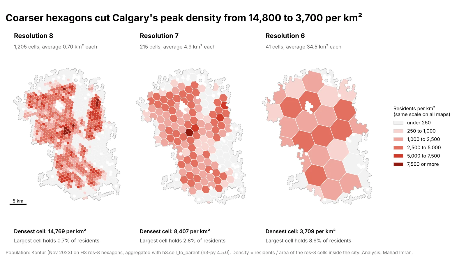
Same population, same colour scale. The densest pockets disappear as cells grow.
| Measure | Resolution 8 | Resolution 7 | Resolution 6 |
|---|---|---|---|
| Cells | 1,205 | 215 | 41 |
| Densest cell (residents per km²) | 14,769 | 8,407 | 3,709 |
| Share of residents in the most populous cell | 0.7% | 2.8% | 8.6% |
| Share of residents living in cells at 5,000+ per km² | 30.6% | 8.0% | 0% |
| Cells fully inside the city | 1,205 | 119 | 8 |
Two findings matter for practice:
- Peaks are the first casualty. At resolution 8, nearly a third of Calgarians live in cells above 5,000 residents per km². At resolution 6, none do. A density threshold, such as an urban service standard or a site screening rule, gives a completely different answer depending on the grid.
- Coarse grids are mostly edge cells. Only 8 of the 41 resolution-6 cells fall fully inside the city. The other 33 are partial, and their density depends on how you treat the missing area.
This is the modifiable areal unit problem: statistics computed on areal units change with the size and placement of those units. It affects every grid and every set of administrative boundaries, and the effect on a map's message is similar to the one I showed for choropleth classification methods. The defence is to choose the resolution for a stated reason and, for important results, check them at a second resolution.
How do you aggregate H3 cells to a coarser resolution?
Map each cell to its parent with cell_to_parent, then group by the parent and sum. The examples below use the H3 v4 API names.
Python (h3-py 4.x and pandas):
import h3
import pandas as pd

# Points to cells: one index column per resolution you need
df = pd.read_csv("incidents.csv")                     # columns: lat, lng
df["h3_9"] = [h3.latlng_to_cell(lat, lng, 9) for lat, lng in zip(df.lat, df.lng)]
df["h3_7"] = df["h3_9"].map(lambda c: h3.cell_to_parent(c, 7))

# Cells to coarser cells: Calgary's res-8 population rolled up to res 6
cells = pd.DataFrame(hexes)                           # columns: id, pop (res 8)
cells["area_km2"] = cells["id"].map(lambda c: h3.cell_area(c, "km^2"))
cells["parent"] = cells["id"].map(lambda c: h3.cell_to_parent(c, 6))

res6 = cells.groupby("parent").agg(pop=("pop", "sum"), area_km2=("area_km2", "sum"))
res6["per_km2"] = res6["pop"] / res6["area_km2"]     # area of the children present
To draw the result, h3.cell_to_boundary(cell) returns the vertices as (lat, lng) pairs, and h3.cells_to_geo(cells) merges a set of cells into one GeoJSON-like outline.
DuckDB with the h3 community extension:
INSTALL h3 FROM community;
LOAD h3;

SELECT h3_cell_to_parent(h3_latlng_to_cell(lat, lng, 9), 7) AS cell,
       count(*) AS incidents
FROM read_parquet('incidents.parquet')
GROUP BY cell
ORDER BY incidents DESC;
DuckDB queries the Parquet file directly, with no import step. The geospatial file formats comparison covers why Parquet suits this kind of table.
PostgreSQL / PostGIS with h3-pg:
CREATE EXTENSION h3;
CREATE EXTENSION h3_postgis CASCADE;

-- geom stored in EPSG:4326
SELECT h3_cell_to_parent(h3_lat_lng_to_cell(geom, 9), 7) AS cell,
       count(*) AS incidents
FROM incidents
GROUP BY cell;
Function names have shifted between h3-pg versions, so check the docs for the version you install. Store the index as the h3index type or a 64-bit integer, index the column, and join other tables on it.
What are the common H3 pitfalls?
- Cells are not equal area. I computed the area of all 288,122 cells at resolution 4: the largest hexagon is 1.97 times the smallest. At city scale the variation is small within a city and larger between cities. Resolution-8 cells average 0.703 km² in Calgary and 0.828 km² in Islamabad, 18% larger. Divide by
h3.cell_area(cell), never by the resolution average, and never by an area measured in Web Mercator, which I covered in why web maps get area wrong. - Pentagons. Each resolution has 12 pentagons with five neighbours and six children. At resolution 8 a pentagon covers 0.372 km², about half an average hexagon. They sit in the oceans, but global analyses should handle them, for example by checking
h3.is_pentagon. - Parents do not exactly contain their children. In Calgary about 7% of the area of resolution-8 cells falls outside the resolution-7 parent they roll up to, and 75 of 1,205 resolution-8 centres lie outside their resolution-6 grandparent. Aggregation by index is consistent, but do not use a parent's outline to clip or select its children.
- Partial cells at the study edge. When a study area boundary cuts through cells, coarse resolutions are mostly partial cells. Decide whether density uses the full cell area or only the part inside the study area, and say which.
- The modifiable areal unit problem. As the Calgary test shows, peaks, thresholds and rankings move with resolution. Report the resolution with every result, and test sensitive conclusions at a second one.
- Splitting counts down. Assigning one seventh of a parent's count to each child assumes an even spread inside the parent. If you need finer detail, find finer source data.
For optimization work such as the coverage curve, resolution sets the demand points the model can see, so it is worth one sensitivity run at the next finer resolution before a final recommendation.
What should you take from this?
Pick the H3 resolution from the size of the decision and the resolution of your source data: 8 for most city work, 9 for walking scale and blocks, 7 for districts, 5 or 6 for regions. Store data finer than you need, aggregate up with cell_to_parent, divide by each cell's real area, and state the resolution next to every number, because Calgary's peak density is 14,769 or 3,709 residents per km² depending on that one choice. For where H3 fits in the wider toolkit, see what location intelligence is.
If you need a hexagon-based analysis set up, or an existing one checked for resolution and area errors, email me at mahad.imran29@gmail.com.