WorldPop, GHS-POP, LandScan, Meta's High Resolution Settlement Layer, Kontur Population and GPWv4 all start from census counts and spread them over a grid, so the right one depends on resolution, method and what "population" means. WorldPop (100 m) and Meta (30 m) map where people live, LandScan (about 1 km) maps a 24-hour average of where people are, and GHS-POP is the best time series. Before using any of them, check the grid's total against the census for the same boundary: Kontur's hexagons came out 9.6% above Islamabad's 2023 census or 3.1% below it, depending only on how the boundary was applied.
This article compares the six datasets on producer, resolution, method, population type, years and licence, then shows a check I ran on the Kontur hexagons used across this site against census figures for Calgary, Islamabad and Bahawalpur, with Python code for zonal sums and census rescaling.
What is a gridded population dataset?
A gridded population dataset is an estimate of how many people live in, or are present in, each cell of a regular grid. Census offices publish counts for administrative units such as districts, tehsils or dissemination areas, which vary in size and change over time. A grid spreads those counts into equal cells, so you can sum people inside any polygon: a drive-time catchment, a flood zone or a station's coverage area.
How the counts are spread is what separates the datasets:
- Areal weighting spreads each unit's count evenly over its area. Simple and transparent, but it puts people in forests and lakes.
- Dasymetric mapping spreads counts according to ancillary data such as built-up area, land cover, roads or night lights, so empty land gets few people.
- Machine-learning models (for example random forests) learn the relationship between those covariates and population density, then predict a weight for every cell.
- Building-based methods detect buildings in satellite imagery and allocate people to cells with buildings.
Almost every dataset is ultimately a census count redistributed. A grid never contains more information about the total than the census behind it, and its error is concentrated in where people are put inside each unit.
How do WorldPop, GHSL, LandScan, Meta, Kontur and GPW compare?
| Dataset | Producer | Resolution | Method | Population type | Years | Licence |
|---|---|---|---|---|---|---|
| WorldPop Global 2 (R2025A) | University of Southampton | 100 m (1 km aggregates) | Random-forest dasymetric, constrained to settlements | Residential | Annual, 2015 to 2030 | CC BY 4.0 |
| GHS-POP R2023A | European Commission Joint Research Centre | 100 m (and 3 arc-seconds) | GPWv4.11 census counts spread by GHSL built-up surface and volume | Residential | Every 5 years, 1975 to 2030 | CC BY 4.0 |
| LandScan Global | Oak Ridge National Laboratory | 30 arc-seconds (about 1 km) | Multi-variable dasymetric, now with machine-learning models | Ambient (24-hour average) | Annual, 2000 onward | CC BY 4.0 since the 2022 public release |
| Meta High Resolution Population Density Maps (HRSL) | Meta and CIESIN, Columbia University | 30 m (1 arc-second) | Buildings detected in satellite imagery, census counts allocated to them | Residential, with age and sex splits | Varies by country | CC BY 4.0 |
| Kontur Population | Kontur | H3 resolution 8 (about 400 m), plus 3 km and 22 km | Fuses GHS-POP, Meta HRSL, Microsoft building footprints, land cover and OpenStreetMap | Residential | Releases to 1 November 2023 | Creative Commons Attribution |
| GPWv4.11 | CIESIN, Columbia University (NASA SEDAC) | 30 arc-seconds | Areal weighting of about 13.5 million census units | Residential | 2000, 2005, 2010, 2015, 2020 | CC BY 4.0 |
A few things the table does not show:
- WorldPop R2025A is labelled an alpha release that may change. WorldPop's older 2000 to 2020 series is still widely cited and is the stable choice for historical work.
- GHS-POP's 2025 and 2030 epochs are projections. Each epoch is a separate estimate on the same grid, which is what makes it good for change over time.
- LandScan counts where people are across a day. A business district gets daytime workers, and a suburb loses them. That is ideal for disaster exposure and wrong for "how many residents live within 2 km of this school".
- Meta's maps are only as current as the imagery and census behind each country. Check the reference year for your country before comparing it with anything else.
- Kontur is a derived product. Its value is that it is already on H3 hexagons with gaps filled from several sources. Its inputs carry their own reference years.
- GPWv4 is the baseline with no ancillary data. It is coarse, but it makes no modelling assumptions, which is useful when you need to separate census error from model error.
Should you use residential or ambient population?
Use residential population for anything about homes and the services people reach from home, and ambient population for anything about who is exposed at an unknown time of day. School and clinic access, voter or customer catchments, and station coverage all assume people start from where they live, so WorldPop, GHS-POP, Meta or Kontur fit. Earthquake, flood and industrial-accident exposure, where the event can happen at 2 pm on a Tuesday, is LandScan's purpose.
Mixing them in one model gives a number nobody can interpret. If you need both, run the analysis twice and report the two answers side by side.
Does a gridded population total match the census?
Usually within a few percent for a whole city, but only if the grid and the census cover the same area, and that is easy to get wrong. I checked the Kontur hexagons (1 November 2023 release, H3 resolution 8) behind the Site Selection Showdown map against census figures for each study area.
Method:
- The study areas are the OpenStreetMap boundaries for the City of Calgary, Islamabad Capital Territory and Bahawalpur City Tehsil, as returned by Nominatim. I measured their areas in each city's UTM zone.
- The site keeps every hexagon that touches the boundary, with its full population. I also computed each hexagon's share of area inside the boundary and weighted its population by that share, which assumes people are spread evenly within a hexagon.
- Census figures: Statistics Canada's 2021 Census for Calgary (1,306,784), and the Pakistan Bureau of Statistics 2023 census for Islamabad Capital Territory (2,363,863 on 906 km²) and Bahawalpur City tehsil (815,202, as compiled from the PBS tehsil tables by City Population).
| Study area | OSM boundary | Hexagons | Every touching hexagon | Weighted by share inside | Census | Difference |
|---|---|---|---|---|---|---|
| Calgary | 852.7 km² | 1,205 | 1,463,328 | 1,456,577 | 1,306,784 (2021) | +12.0% / +11.5% |
| Islamabad Capital Territory | 962.8 km² | 1,164 | 2,590,233 | 2,291,566 | 2,363,863 (2023) | +9.6% / −3.1% |
| Bahawalpur City Tehsil | 399.0 km² | 542 | 673,192 | 604,230 | 815,202 (2023) | −17.4% / −25.9% |
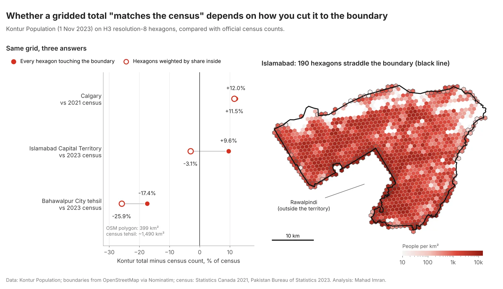
Each city tells a different story about why a grid total and a census figure disagree.
Each row shows a different failure:
- Islamabad: the boundary rule. 190 of the 1,164 hexagons cross the territory line, and they hold 514,217 people. Most of those crossing the southern edge are in dense Rawalpindi, which presses right against the boundary. Counting them in full adds about 299,000 people who live outside the territory. Weighting by area brings the total to 3.1% below the census, which is a good match for a modelled grid.
- Calgary: the reference year. The boundary barely matters here (198 crossing hexagons hold only 23,559 people, and weighting changes the total by 0.5%). The gap is time. Calgary grew fast after 2021, and the City of Calgary's own estimate for April 2023 was 1,422,800, within about 3% of the Kontur total. Comparing a 2023 grid with a 2021 census makes a good grid look 12% wrong.
- Bahawalpur: the boundary does not match the census unit. The OpenStreetMap polygon called Bahawalpur City Tehsil covers 399 km². Compilations of the census tables put the tehsil at about 1,490 km². The 2023 figure usually quoted for the city itself is 903,795. None of these covers the same area as the polygon, so the −17% and −26% come from mismatched boundaries and cannot be used to judge Kontur's accuracy.
The general rule: before you use any gridded dataset, sum it over a boundary that matches a census unit exactly, for the same reference year, and explain any gap larger than a few percent before running the analysis.
How do you sum a population raster inside polygons in Python?
Read the raster with rasterio, check its CRS and nodata value, then use zonal statistics to sum the cells inside each polygon. The choice of tool matters at the edges.
import geopandas as gpd
import rasterio
from rasterstats import zonal_stats
from exactextract import exact_extract

tif = "worldpop_pakistan_2023_100m.tif"      # a WorldPop country GeoTIFF
with rasterio.open(tif) as src:
    print(src.crs, src.res, src.nodata)       # EPSG:4326, ~0.000833°, nodata
    pop = src.read(1, masked=True)            # masks the nodata cells
    print(f"Raster total: {pop.sum():,.0f}")

zones = gpd.read_file("tehsils.gpkg").to_crs(src.crs).reset_index(drop=True)

# Centre-of-cell rule: a cell counts in full if its centre is inside
zs = zonal_stats(zones, tif, stats=["sum"], all_touched=False)
zones["pop_centre_rule"] = [z["sum"] for z in zs]

# Exact fractional coverage: each cell weighted by its share inside
ee = exact_extract(tif, zones, "sum", include_cols=["tehsil_code"], output="pandas")
zones = zones.merge(ee.rename(columns={"sum": "pop_exact"}), on="tehsil_code")
Use exactextract for small or irregular polygons, where a 100 m cell is a large share of the shape. With all_touched=True, rasterstats counts every cell the polygon touches in full, which is the raster version of the Islamabad mistake above.
How do you rescale a gridded dataset to census totals?
Multiply every cell in a census unit by the ratio of the census count to the grid's sum for that unit. This keeps the grid's pattern inside each unit and makes every unit total match the official figure.
import numpy as np
import rasterio
from rasterio import features

with rasterio.open(tif) as src:
    pop = src.read(1, masked=True).filled(0).astype("float64")
    zone_id = features.rasterize(
        zip(zones.geometry, zones.index + 1), out_shape=pop.shape,
        transform=src.transform, fill=0, dtype="int32")
    profile = src.profile

grid_sum = np.bincount(zone_id.ravel(), weights=pop.ravel())
factor = np.ones_like(grid_sum)
factor[zones.index + 1] = zones["census_2023"].to_numpy() / grid_sum[zones.index + 1]
adjusted = pop * factor[zone_id]

profile.update(dtype="float32", nodata=-1)
with rasterio.open("pop_rescaled_2023.tif", "w", **profile) as dst:
    dst.write(adjusted.astype("float32"), 1)
Rescale with the smallest census units you can match exactly. A factor far from 1 in one unit (say below 0.8 or above 1.25) is worth a look before you trust it: it usually means a boundary mismatch, a new development the model missed, or an error in the census join. To move the result onto hexagons, aggregate with H3 at a resolution that suits the analysis, as covered in the H3 resolution guide.
Which population dataset should you use?
| Job | Use | Why |
|---|---|---|
| Access to schools, clinics or shops at neighbourhood scale | WorldPop 100 m or Meta 30 m, rescaled to census | Residential, fine enough for walking distances |
| Ready-made hexagons for site selection or coverage models | Kontur Population | Already on H3; check boundary and year first |
| Change over decades, urban growth | GHS-POP | Consistent method across 1975 to 2030 |
| Disaster exposure, daytime presence | LandScan Global | Ambient population |
| Age or sex groups (women of reproductive age, children under 5) | Meta's demographic layers, or WorldPop age-sex grids | Splits by group |
| A baseline with no model assumptions | GPWv4.11 | Census spread by area only |
| Official counts for a report | The census itself | Grids are estimates |
For Pakistan specifically, the 2023 census, the country's first digital census, recorded 241.49 million people and publishes counts down to tehsil level. That makes rescaling straightforward, and it matters: grids built before the 2023 results were released relied on older census figures and projections. The Islamabad school access study on this site used Kontur hexagons for the same reason the site selection maps do: they are ready to route on. The same caution applies there. A population grid sets the denominator for every accessibility ratio, including the supply-to-demand ratios in two-step floating catchment analysis, so an error in the grid passes straight into the result.
What should you take from this?
Pick the dataset by what you need to count: residents at fine scale (WorldPop, Meta), residents over time (GHS-POP), people present during the day (LandScan), or hexagons ready for analysis (Kontur). Then check it against the census for the exact same boundary and year. In my three cities, the boundary rule moved Islamabad's total by 13 percentage points, the reference year explained Calgary's 12% gap, and in Bahawalpur the boundary itself was not the census unit. None of that showed up on the map. The same checks belong in any fire station or service-coverage study before the first model runs.
If you need population estimates prepared and checked for a planning, site-selection or coverage project, email me at mahad.imran29@gmail.com.