Fire station location analysis models the drive time from every candidate site to every place that generates emergencies, then uses an optimization model to choose sites. Set covering finds the fewest stations that reach everyone within a time standard, maximal covering reaches the most people with a fixed number of stations, and p-median minimizes the average response time.
This article explains the three models, the NFPA 1710 travel-time benchmarks they are usually run against, why network drive time beats a radius, and a worked example on Calgary that compares optimized placement with naive placement for several station counts.
What is fire station location analysis?
Fire station location analysis is a location-allocation problem. It has four ingredients:
- Demand: where emergencies happen or where people live. Incident history from computer-aided dispatch (CAD) is the best measure; a population grid is the usual substitute.
- Candidate sites: places a station could actually be built. Existing stations are usually fixed, and the model chooses among new or relocated sites.
- Travel-time matrix: drive time from every candidate to every demand point along the road network.
- A standard: the time within which a demand point counts as "covered", for example 240 seconds of travel.
The output is a set of sites, plus what that set achieves: the share of population or incidents within the standard, the average travel time and the worst-served areas.
What response time is a station supposed to deliver?
Response time is made of parts, and the location model only controls one of them. NFPA 1710 (2020 edition) sets these objectives for career departments:
| Component | NFPA 1710 (2020) objective |
|---|---|
| Turnout time, fire and special operations | 80 seconds |
| Turnout time, EMS | 60 seconds |
| Travel time, first engine company at a fire | 240 seconds or less |
| Travel time, second company (minimum 4 staff) | 360 seconds or less |
| Travel time, initial full alarm assignment (not high-rise) | 480 seconds or less |
| Travel time, unit with AED or higher at a medical call | 240 seconds or less |
| Performance objective | Not less than 90 percent for each turnout and travel objective |
The 240-second first-engine travel benchmark is the one most station studies plan around, because it is the one station location changes. Turnout time is about the station's layout and the crew, and alarm handling is about the dispatch centre. NFPA's NFPA 1710 page notes that the standard has been combined into the consolidated NFPA 1750, with the 2020 edition as the last stand-alone version. Volunteer and combination departments use NFPA 1720 instead, which sets staffing and response objectives by type of area rather than a single travel time.
These are NFPA's objectives, not law, and local targets differ. Calgary's Council-approved target, in its March 2026 fire capital needs assessment, is a first-in engine within 7 minutes at fire and rescue incidents, 90 percent of the time, and the full effective response force within 11 minutes. In the US, ISO's Fire Suppression Rating Schedule uses a distance test instead: full distribution credit needs a first-due engine within 1.5 road miles and a ladder or service company within 2.5 road miles, with an NFPA 1710 performance evaluation accepted as an alternative.
Set covering vs maximal covering vs p-median: which model answers which question?
Each model answers a different planning question. Picking the wrong one is the most common mistake in a station study.
| Model | Question it answers | Objective | Fixed input | Origin |
|---|---|---|---|---|
| Location set covering (LSCP) | How many stations do we need to meet the standard everywhere? | Minimize the number of stations | Coverage standard (all demand covered) | Toregas, Swain, ReVelle and Bergman, 1971 |
| Maximal covering (MCLP) | Where should our N stations go? | Maximize demand covered within the standard | Number of stations | Church and ReVelle, 1974 |
| p-median | Where should N stations go to make the average trip shortest? | Minimize demand-weighted average travel time | Number of stations | Hakimi, 1964 |
Set covering (LSCP)
Set covering finds the smallest set of sites such that every demand point is within the standard of at least one station. Written as an integer program, with binary x_i = 1 if a station opens at site i, and N_j = the sites that reach demand point j within the standard:
minimize    sum_i x_i
subject to  sum_{i in N_j} x_i >= 1     for every demand point j
            x_i in {0, 1}
Its weakness is that every demand point counts the same. A hamlet of 30 people at the city edge can force a whole extra station. In practice planners relax it to "cover at least 90%" or "cover 100% of incidents in the urban service area".
Maximal covering (MCLP)
Maximal covering accepts that the budget is fixed, say five stations, and places them to cover as much demand as possible. With a_j = demand at point j, and y_j = 1 if j is covered:
maximize    sum_j a_j * y_j
subject to  y_j <= sum_{i in N_j} x_i   for every demand point j
            sum_i x_i = p
            x_i, y_j in {0, 1}
Its weakness is the mirror image of set covering: anything outside the standard counts as zero, whether it is 10 seconds or 10 minutes outside. MCLP will happily leave a district far from any station if that buys more coverage elsewhere.
p-median
p-median ignores the standard and minimizes the demand-weighted average travel time across everyone. It tends to produce more even service and a shorter worst case than MCLP, at the cost of covering fewer people within the standard. It is the right model when the question is efficiency rather than compliance, for example placing a new EMS post.
Why does drive time beat a radius for station coverage?
A circle assumes you can drive in a straight line in every direction. Real streets add detours around rivers, rail yards and freeways, cul-de-sac suburbs add distance, and one-way pairs add more. A radius overstates coverage, and it overstates it unevenly: it is most wrong in exactly the areas with the poorest street connectivity.
The Calgary model below makes the size of the error concrete. I chose 20 station sites by maximizing coverage inside 2.4 km circles (1.5 miles, ISO's engine distance applied as a straight line, which is a common shortcut). The circles claimed 79.8% of residents were covered. Measured on the road network, only 28.0% were within a 4-minute drive of those same 20 sites. The same idea applies to retail trade areas, which I cover in drive-time vs radius trade areas.
ISO's own test is road miles, not radius, so even an ISO-oriented study should measure along the network.
Worked example: how many stations does Calgary need, and does optimization matter?
This example uses the same data as my interactive Site Selection Showdown game, where you place fire stations in Calgary and two other cities and compare your placement with the optimal one. It is a planning model of residents, not an assessment of the Calgary Fire Department's actual coverage, which depends on incident data, staffing and existing stations that the model does not include.
Data and method
- Demand: Kontur Population for Canada (1 November 2023 release), on H3 resolution-8 hexagons of about 0.74 km² each. The 1,205 hexagons touching Calgary's OpenStreetMap boundary hold 1,463,328 people and cover a city of about 853 km².
- Network: the OpenStreetMap drive network for Calgary plus a 2 km buffer (38,404 nodes, 90,291 directed edges). Each road class gets a free-flow speed fitted against the OSRM routing engine's car profile: motorway 70, trunk 50, primary 55, secondary 45, tertiary 35, ramps 40 and local streets 22 km/h. The gap from a hexagon's centre to its nearest road is added at 15 km/h.
- Candidate sites: 1,114 hexagons where a station could plausibly go: a drivable road crosses the hexagon and no more than half of it is park, forest, water, military land or airport.
- Models: MCLP and LSCP solved exactly with PuLP and the CBC solver (every MCLP run reported a proven optimum, most in about a second); p-median with a Teitz-Bart vertex-substitution heuristic, a standard approximate method.
- Naive baseline: population-weighted k-means. Cluster the residents into k groups and put a station at the buildable hexagon nearest each cluster centre. That is a sensible way to "put stations where the people are" without an optimizer. I ran it with 10 random seeds and report the median.
Two standards are tested: 4 minutes of drive time, matching NFPA 1710's 240-second first-engine travel benchmark, and 12 minutes, the rule used in the game.
Result 1: optimized vs naive placement
At the NFPA-style 4-minute standard:
| Stations | MCLP optimum | Naive (k-means, median of 10) | Extra residents covered by optimizing |
|---|---|---|---|
| 5 | 18.8% | 6.2% | about 185,000 |
| 10 | 30.6% | 14.5% | about 236,000 |
| 20 | 48.1% | 29.4% | about 274,000 |
| 30 | 60.2% | 41.0% | about 282,000 |
| 40 | 69.2% | 48.9% | about 298,000 |
At the 12-minute game standard:
| Stations | MCLP optimum | Naive (k-means, median of 10) |
|---|---|---|
| 1 | 28.1% | 26.0% |
| 2 | 49.8% | 35.4% |
| 3 | 68.9% | 53.1% |
| 4 | 83.6% | 75.4% |
| 5 | 90.3% | 80.1% |
With a single station the optimizer barely beats putting it at the population centre. From two stations on, the gap opens to 8 to 20 percentage points, and at the 4-minute standard it is worth roughly the population of a large suburb at every station count tested. Put differently, the naive 40-station layout (48.9%) covers about what 20 optimized stations achieve (48.1%).
The reason is overlap. k-means puts each station in the middle of its own cluster of people and never checks whether two stations' drive-time areas overlap or whether a cluster's centre sits next to a freeway that extends its reach. MCLP sees the whole travel-time matrix at once.
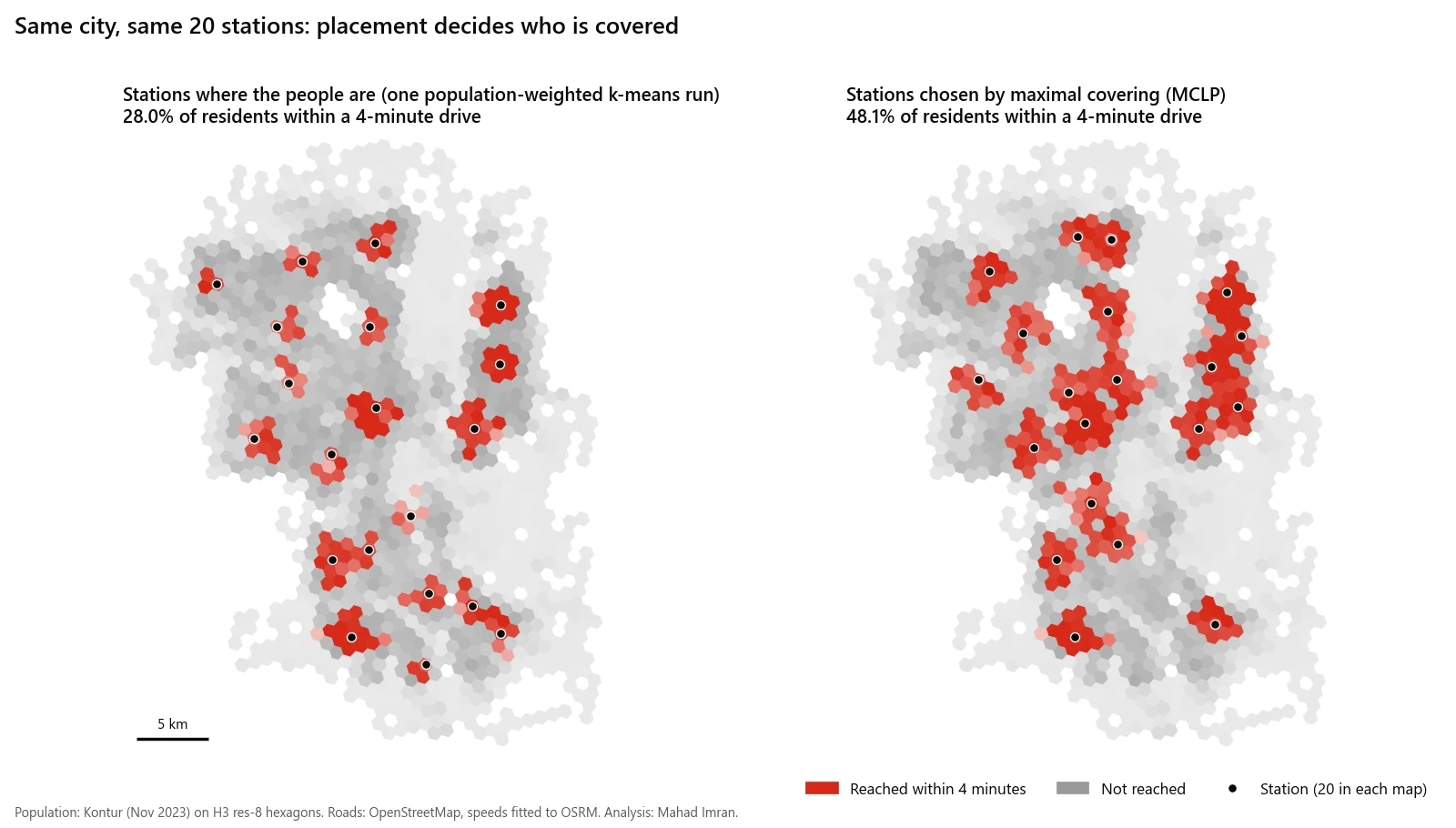
Twenty stations each way at the 4-minute standard. The k-means panel is a single run (28.0%); the table above reports the median of 10 runs (29.4%).
Result 2: what each coverage target costs (set covering)
Fewest stations needed, from LSCP, to reach a share of residents:
| Target share of residents | Within a 4-minute drive | Within a 12-minute drive |
|---|---|---|
| 80% | 57 | 4 |
| 90% | 79 | 5 |
| 95% | 101 | 6 |
| Every populated hexagon that can be reached | 342 (99.91%) | 39 (99.99%) |
This table is the strongest argument for writing the coverage target down before anything else. Going from 95% to full coverage at 12 minutes takes the station count from 6 to 39. At 4 minutes it goes from 101 to 342, and 34 hexagons with 1,285 residents cannot be reached within 4 minutes from any buildable site at all. The last few percent are fringe areas with very few people per square kilometre, and serving them to the same standard costs more than the whole core.
It also shows how much the standard matters. In this model a 4-minute standard needs roughly 14 times as many stations as a 12-minute one for the same 80% target. A study that does not state its standard and its target share cannot be compared with another one.
Result 3: maximal covering vs p-median
The two models disagree in a useful way:
| Scenario | Model | Covered within standard | Average drive time | 90th percentile drive time |
|---|---|---|---|---|
| 20 stations, 4-minute standard | MCLP | 48.1% | 4.9 min | 9.0 min |
| 20 stations, 4-minute standard | p-median | 42.4% | 4.6 min | 7.2 min |
| 4 stations, 12-minute standard | MCLP | 83.6% | 9.2 min | 14.0 min |
| 4 stations, 12-minute standard | p-median | 76.7% | 9.0 min | 14.0 min |
Times are population-weighted and capped at 30 minutes. With 20 stations, MCLP covers 5.7 points more people within 4 minutes, but its 90th-percentile resident waits 1.9 minutes longer, because MCLP gives no credit for getting an uncovered neighbourhood from 12 minutes down to 6. NFPA 1710 measures the 90th percentile of incidents, so a department reporting against it should look at both numbers, not only the MCLP coverage figure.
Result 4: what a radius would have told you
| Stations | Coverage claimed by 2.4 km circles | Actual coverage within a 4-minute drive (same sites) | MCLP on the network |
|---|---|---|---|
| 10 | 49.6% | 17.6% | 30.6% |
| 20 | 79.8% | 28.0% | 48.1% |
| 40 | 99.6% | 40.4% | 69.2% |
The radius study is wrong twice. It overstates its own coverage by a factor of two to three, and its chosen sites are worse than network-optimized ones even when both are measured properly.
If you want to feel these trade-offs rather than read them, the Site Selection Showdown lets you place three stations in Calgary under the 12-minute rule and then reveals the 68.9% optimum from the table above.
What data does a real station study need?
The Calgary example uses open data. A study a city would act on needs more:
- Incident history. Three to five years of geocoded CAD incidents, by type and time of day. NFPA's 90 percent objective is measured against incidents, not residents, and incidents cluster differently from population (highways, downtown, care homes).
- Calibrated travel speeds. Apparatus GPS (AVL) records give real speeds by road class and time of day. Free-flow car speeds, as used above, are optimistic for heavy apparatus in some places and pessimistic where crews run with lights and sirens.
- Turnout time per station. Measured, not assumed, because 80 seconds versus 120 seconds at one station changes its effective travel budget.
- Existing stations as fixed sites. Most real questions are "where does the next station go" or "which station should move", which means solving with current stations locked in.
- Real candidate sites. City-owned parcels, zoning, and access to arterials in both directions.
- Growth. Planned subdivisions over the life of a station, which is typically decades.
- Clean addresses and centerlines. Incident geocoding and network routing depend on the same road centerline data that NG911 relies on, which I cover in the NG911 readiness checklist.
Limitations of coverage models
Coverage models are a decision aid, not an answer. Know where they break.
- Coverage is binary. A point 4:01 away counts the same as one 20 minutes away under MCLP and LSCP. Always report the travel-time distribution alongside coverage.
- Stations are assumed available. If the first-due engine is already on a call, the next one is further away. Busy systems need backup or double-coverage formulations, or a simulation, rather than single coverage.
- Free-flow travel. The Calgary model has no congestion and no time-of-day effects, and it is calibrated to a car routing profile, not to fire apparatus.
- Residents are where they sleep. A population grid puts people at home. Daytime demand downtown and in industrial areas is much higher than residential counts suggest.
- Hexagon aggregation. Everyone in a 0.74 km² hexagon is placed at its centre. That is coarse for a 4-minute standard, where a few hundred metres matter, and a parcel- or address-level demand layer is better for final siting.
- Politics and land. The optimizer does not know which parcels are for sale, which neighbourhoods were promised a station, or what a site costs. Use it to compare options and to show the cost of each coverage target, then decide.
If you want a coverage study for your department or municipality, built on your incident data and network, email me at mahad.imran29@gmail.com.