
A drive-time trade area counts the people who can reach a site within a set number of minutes on the road network. A radius counts everyone within a straight-line distance. Across 169 Calgary sites, a 3-mile ring and a 10-minute drive enclosed similar land, but their population counts differed by more than 25% at 42% of sites.
This article covers that comparison in full, why the ring goes wrong, when a ring is still the right tool, where to get isochrones, how traffic changes the answer, and how to count people inside a polygon using US and Canadian census units.
Drive time vs radius trade area: what is the difference?
A radius trade area (or ring) is a circle of fixed distance around a site, such as 1, 3 or 5 miles. It is simple, cheap and easy to explain to a real estate committee.
A drive-time trade area (an isochrone, or a service area in Esri's terminology) is the set of places from which a driver can reach the site within a fixed time, such as 10 minutes, travelling along the road network at modelled speeds.
The difference is that a ring ignores everything that shapes how people actually arrive:
- Barriers. Rivers, rail yards, freeways without interchanges, parks and airports cut neighbourhoods off from a site that looks close on a map.
- Corridors. A freeway or arterial stretches the catchment along its length, pulling in people well beyond the ring.
- Network gaps. Curvilinear suburbs with few entry points add minutes that straight-line distance cannot see.
For a site that will cost real money, the question is how much these effects change the answer. The rest of this article measures it.
How different are a 3-mile ring and a 10-minute drive in practice?
I tested this on Calgary, using the same data behind the Site Selection Showdown game on this site.
The data and method
- Population: Kontur Population, a modelled grid of H3 hexagons at resolution 8 (about 400 m across). Clipped to the City of Calgary, that is 1,205 hexagons of about 0.7 km² each, holding 1,463,328 people.
- Road network: the OpenStreetMap drive network for the city plus a 2 km buffer (38,404 nodes and 90,291 directed edges), with one speed per road class. The speeds were fitted so that trips under 20 minutes match the OSRM car profile at the median. OSRM is a free-flow model, so these are uncongested times.
- Drive time: measured inbound, from the centre of every hexagon to the candidate site, because shoppers drive to the store.
- Candidate sites: every hexagon that has a drivable road and is not mostly park, water, forest or airfield, and whose surroundings within 7 km lie inside city limits. That leaves 169 sites, and keeps the city edge from shrinking either shape.
- Ring: 3 miles is 4.83 km, so the ring covers 73.2 km² (28.3 square miles). A hexagon counts as inside if its centre is.
Matching the reach fairly
Comparing a ring with a drive time is only fair if the two cover a similar amount of ground. Across the 169 sites, the median free-flow catchment was:
| Drive time | Median catchment area | Median population reached |
|---|---|---|
| 8 minutes | 35.3 km² | 80,850 |
| 9 minutes | 48.7 km² | 116,491 |
| 10 minutes | 65.6 km² | 161,865 |
| 11 minutes | 86.9 km² | 208,490 |
| 12 minutes | 110.1 km² | 265,219 |
A 3-mile ring (73.2 km²) sits between the 10- and 11-minute catchments, so the comparison below pairs a 3-mile ring with a 10-minute drive. In Calgary at free-flow speeds they are about the same size.
Results across 169 sites
| Measure | Result |
|---|---|
| Median ratio, ring population ÷ drive-time population | 1.01 (they agree on average) |
| Middle 80% of sites | 0.76 to 2.17 |
| Sites where the two counts differ by more than 25% | 42% |
| Sites where they agree within 10% | 24% |
| Sites where the ring overstates by more than 25% | 33% |
| Sites where the ring understates by more than 25% | 9% |
| Median share of the ring's people who are more than 10 minutes away | 19% |
| Median share of the drive-time's people who are outside the ring | 15% |
| Rank correlation between the two (Spearman) | 0.78 |
| Sites shared by the top 10 under each method | 4 of 10 |
The headline is not that rings are biased. On average they land close. The problem is that the error is large and unpredictable for any single site, and site selection is always about a single site.
The ranking result matters most. If you shortlisted the top 10 Calgary sites by 3-mile ring population, only 4 of them would also be in the top 10 by 10-minute drive-time population. The single best site by drive time, on 16 Avenue NE (the Trans-Canada Highway) in the inner northeast, ranks 72nd of 169 by ring population. It reaches 307,647 people in 10 minutes, but only 175,863 live within 3 miles of it. The freeway carries its catchment well past the ring.
Six example sites
These are the buildable hexagons nearest to six well-known Calgary locations. Population is counted inside city limits only.
| Site | 3-mile ring | 10-minute drive | In both | Ring only | Drive only | Ring ÷ drive |
|---|---|---|---|---|---|---|
| Downtown core | 221,230 | 279,477 | 218,190 | 3,040 | 61,287 | 0.79 |
| Chinook Centre | 168,260 | 237,115 | 160,570 | 7,690 | 76,545 | 0.71 |
| Sunridge (northeast) | 191,725 | 210,737 | 177,340 | 14,385 | 33,397 | 0.91 |
| Southcentre | 150,467 | 153,185 | 122,428 | 28,039 | 30,757 | 0.98 |
| Crowfoot (northwest) | 166,853 | 156,447 | 124,468 | 42,385 | 31,979 | 1.07 |
| Market Mall (northwest) | 170,436 | 119,460 | 101,724 | 68,712 | 17,736 | 1.43 |
Three patterns show up:
- Arterial sites are undercounted by rings. Chinook Centre sits on Macleod Trail near Glenmore Trail. The ring misses 76,545 people who can drive there in 10 minutes, a third of the true catchment.
- Sites hemmed in by barriers are overcounted. At Market Mall the ring includes 68,712 people, mostly south of the mall, who cannot reach it within 10 minutes. The ring overstates the market by 43%.
- Matching totals can hide a different market. Southcentre's ring and drive time differ by less than 2% in total population, which looks like agreement. But 58,796 people are in one area and not the other, 38% of the drive-time population. At Crowfoot the totals are within 7% and 74,364 people differ. If you then profile income, age or household size, you are describing partly the wrong neighbourhoods.
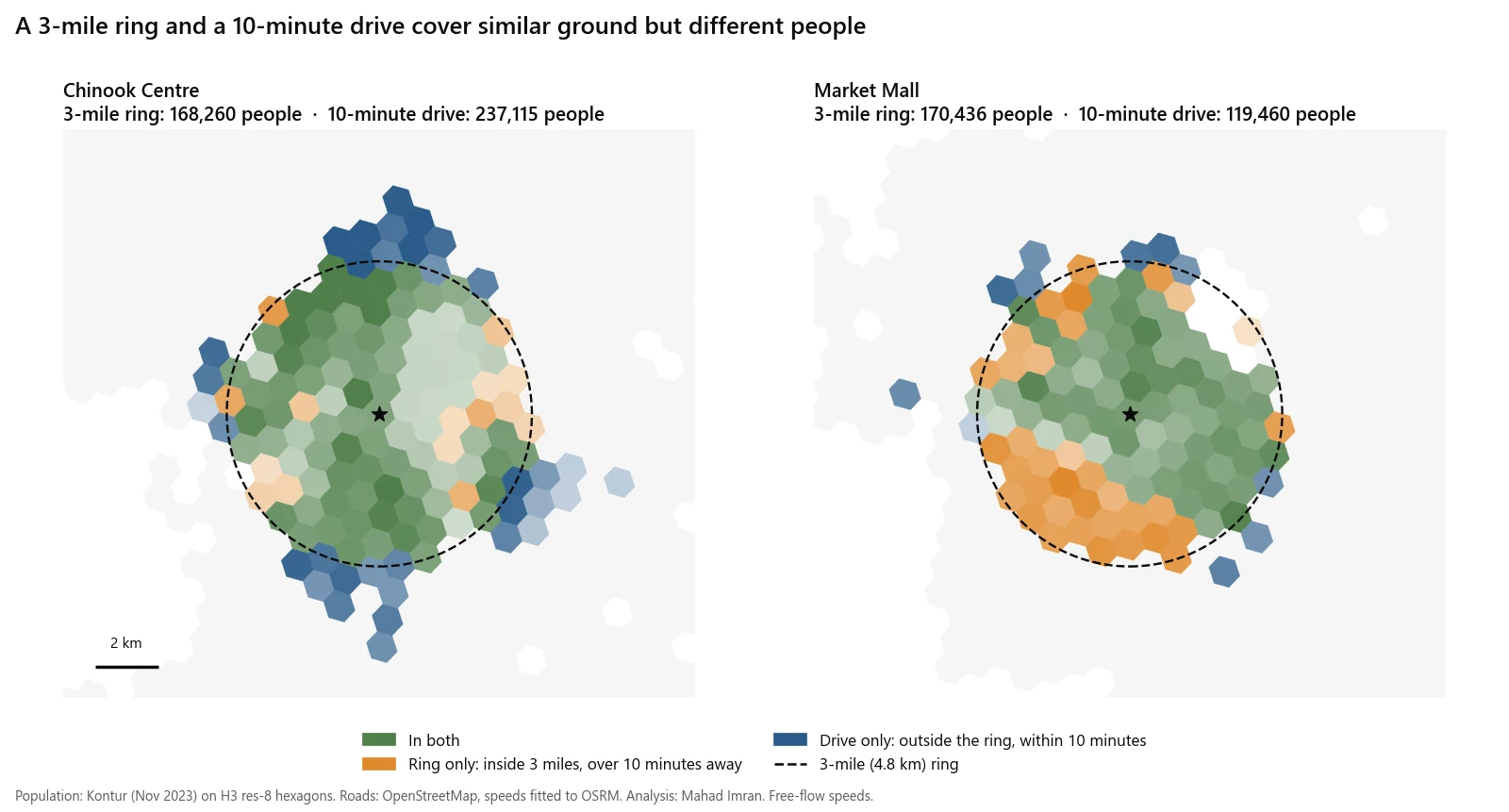
Chinook Centre and Market Mall: green is in both areas, orange only in the ring, blue only in the drive time.
Is it just the ring's size?
To check whether a better-sized ring would fix this, I drew a second ring at every site with exactly the same area as that site's own 10-minute catchment. This removes size from the comparison and leaves only shape.
| Measure (ring sized to each site's own catchment) | Result |
|---|---|
| Median ratio, ring ÷ drive-time population | 0.92 |
| Sites off by more than 25% | 6.5% |
| Median share of people in one area but not the other, relative to the drive-time population | 33% |
| Sites where that mismatch exceeds 20% | 80% |
A perfectly sized ring fixes the totals at most sites. It does not fix the people. At four out of five sites, more than a fifth of the population is still on the wrong side of the line. You can only size a ring this way after computing the drive time anyway, so in practice there is no shortcut.
When is a radius trade area good enough?
Rings are not wrong everywhere. They are the right choice when:
- The boundary is legal, not behavioural. Lease radius restrictions and many franchise territories are written as distances. If the contract says 3 miles, analyse 3 miles. See franchise territory mapping for how those boundaries should be drawn.
- You are screening, not deciding. For a first pass over hundreds of candidate sites, rings are fast and consistent. The Spearman correlation of 0.78 above says rings sort sites roughly right. Run drive times on the shortlist.
- The street grid is dense and even. Rings fail where networks are uneven. In this test the gridded downtown core was the one place where almost everyone inside the ring, all but 3,040 people, was also inside the 10-minute drive.
- You must match a benchmark. If a lender, landlord or an existing store-performance model uses 1-3-5 mile rings, report rings alongside drive times so the numbers are comparable.
Use drive time when the decision commits capital to a specific site, when the site sits near a freeway, river, rail line or large park, or when you will profile the people inside the area and not just count them.
Where do drive-time isochrones come from?
Four common sources, with what each actually does:
| Source | Isochrone support | Traffic | Notes |
|---|---|---|---|
| OSRM | No isochrone endpoint. Services are route, nearest, table, match, trip and tile. | Free-flow speeds from the routing profile, unless you load your own segment speed files | Fast and open source. Build catchments from the table service or a precomputed grid, as in the Calgary test. |
| Valhalla | Native isochrone endpoint. Contour times in minutes, up to four contours by default. | Accepts a date_time for a departure or arrival time | Open source, OpenStreetMap based. Check what speed data your routing tiles were built with before reading anything into time of day. |
| Esri ArcGIS Network Analyst | Service area analysis | Time of day and date are used for traffic when the network dataset or service includes traffic data | Commercial. Esri's Business Analyst extension adds a Huff model tool on the same platform. |
| HERE Isoline Routing API v8 | Native isolines by time or distance | departureTime sets the start time. departureTime=any ignores traffic. | Commercial. Useful when you need traffic-aware catchments by hour. |
Whichever you use, write down the engine, the date of the road data, the speed assumptions and the time of day in the report. Two analysts using different engines will draw different polygons for the same site, and the committee should know which one it is looking at.
Should you use rush-hour or free-flow drive times?
Free-flow catchments are the largest a site will ever have. They flatter every location, and they flatter freeway sites most because freeways gain the most speed when traffic is light.
The Calgary numbers above are free-flow. That is a fair basis for comparing a ring with a drive time, because both are idealised. It is not a fair basis for forecasting sales at a site whose customers arrive at 5:30 pm on a weekday.
A practical rule:
- Pick the hour that matters. Grocery and big-box peak on weekends. Quick-service dinner trade is weekday evening. Childcare and schools are weekday morning drop-off.
- Compute the catchment at that hour with a traffic-aware engine, using historical traffic for a typical week, not live traffic on the day you ran it.
- Keep a free-flow version as the upper bound, and report both. The gap between them is itself useful: a site whose catchment collapses at peak is more exposed to congestion than one that barely changes.
Drive-time catchments are also used for public services. The same method, solved for coverage, is how fire station location analysis is done.
How do you count population inside a trade area in the US and Canada?
The polygon is only half the job. You then need people, households and spending inside it, which means overlaying it on census units.
| United States | Canada | |
|---|---|---|
| Distance unit in reports | Miles | Kilometres |
| Main small-area unit | Block group | Dissemination area (DA) |
| Typical size | About 600 to 3,000 people | Average of 400 to 700 people |
| Detailed demographics from | American Community Survey 5-year estimates. Block groups are the smallest published ACS geography, for select tables. | Census of Population. The DA is the smallest standard area for which all census data are disseminated. |
| Postal geography | ZIP Code Tabulation Areas, built from census blocks to approximate ZIP codes | Census forward sortation areas, the first three characters of the postal code |
Apportioning units the boundary cuts
A drive-time polygon will slice through block groups and DAs. There are three ways to handle the cut units, in increasing order of accuracy:
- Centroid rule. Include a unit if its centre is inside. Fast, but can swing totals by thousands at the edge.
- Area weighting. Include the share of the unit's population equal to the share of its area inside the polygon. This assumes people are spread evenly, which is false wherever a unit contains a park, an industrial strip or undeveloped land, which describes most suburban edge units.
- Dasymetric weighting. Spread each unit's population over its residential land or building footprints first, then intersect. This is the method to use when a few thousand people decide the answer.
DA counts come from the census of the reference year, so in fast-growing suburbs check building permits or newer population estimates before trusting them. ACS block group figures are five-year estimates with margins of error, and those margins matter when a trade area contains only a handful of block groups.
What are the limitations of this comparison?
- Modelled population. Kontur is a modelled grid, not a census count, and it was clipped to city limits. People just outside the boundary, for example in Chestermere, are not counted in either shape.
- Free-flow speeds. Speeds were fitted to OSRM, which has no congestion. Peak-hour catchments would be smaller, and smaller by different amounts at different sites.
- Hexagon resolution. Hexagons are about 0.7 km². Membership is decided by the hexagon's centre, which blurs both boundaries by a few hundred metres.
- One city. Calgary has a freeway ring road, a river valley and large parks. A flat grid city would likely show smaller differences and a city cut by water would show larger ones. Test before generalising.
- Population is not sales. A trade area tells you who can reach a site, not who will choose it. Competition and store attractiveness come next, which is what a gravity model handles. See retail site selection with GIS for the full method, including a worked Huff model.
What should you do with this?
If you are comparing sites for a lease or a franchise rollout, run drive times at the hour your customers travel on every shortlisted site, keep rings only where a contract or benchmark needs them, and profile the people inside the drive-time polygon, not the ring. When ring and drive time disagree by more than about a quarter, find out why on the map before the committee meeting, because someone will ask.
If you need drive-time trade areas built for your candidate sites, scoped or done, email me at mahad.imran29@gmail.com.