The two-step floating catchment area (2SFCA) method measures access to a service as the supply available per resident. It divides each facility's capacity by the population that can reach it, then gives every neighbourhood the sum of those ratios for the facilities in its reach. In an illustrative Islamabad test with 12 hypothetical clinics, 310,413 residents lived within 2 km of a clinic yet scored below the median, because the clinics near them served the most people.
This article compares the common measures of spatial accessibility, explains 2SFCA and its enhanced version (E2SFCA), and works through a full example on Islamabad's population grid, with Python code. The clinics in the example are hypothetical, placed by a stated rule so the method can be shown on real population data.
What are the main ways to measure spatial accessibility?
Spatial accessibility measures how easily people in one place can reach a service, given where the service is, how much of it there is and how many other people want it. The common measures differ in which of those three things they count:
| Measure | What it gives each area | Counts facility size? | Counts competing demand? | Distance treatment | Islamabad test result |
|---|---|---|---|---|---|
| Nearest-facility distance | Distance or time to the closest facility | No | No | Continuous | Median resident 3.5 km away |
| Cumulative opportunities | Facilities (or doctors) within X km or minutes | Yes | No | Hard cut-off | Median covered resident: 16 doctors within 6 km |
| Coverage | Inside or outside a service standard | No | No | Hard cut-off | 80.7% of residents within 6 km |
| Gravity (Hansen) | Sum of supply, weighted down by distance | Yes | No | Smooth decay | Not computed here |
| 2SFCA | Supply-to-population ratio within reach | Yes | Yes | Hard cut-off | Median 5.6 doctors per 100,000 |
| E2SFCA | 2SFCA with distance-decay weights | Yes | Yes | Stepped decay | Median 5.7 doctors per 100,000 |
The first three are what most GIS projects report. They answer "how far?" and "how many people are inside the line?", which is the right question for emergency services, where the coverage curve and the station location models are built around a response-time standard.
They miss one thing that matters for clinics, hospitals, schools and childcare: capacity runs out. A clinic 500 m away that serves 400,000 people offers less than a clinic 3 km away that serves 90,000. The gravity model counts facility size but ignores competition. The floating catchment family counts both.
What is the two-step floating catchment area method?
2SFCA computes access in two steps, each using a catchment of the same size (a distance or travel time d0):
Step 1. For each facility j, find all population locations k within d0 and compute a supply-to-demand ratio:
Rj = Sj / Σ Pk (for all k with dkj ≤ d0)
where Sj is the facility's capacity (doctors, beds, appointment slots) and Pk is population.
Step 2. For each population location i, find all facilities within d0 and add up their ratios:
Ai = Σ Rj (for all j with dij ≤ d0)
Ai reads like a local provider-to-population ratio: doctors per 100,000 residents, available to the people in that place.
The method was named and formalised by Luo and Wang (2003) in Environment and Planning B, building on earlier work by Radke and Mu (2000). Luo and Wang applied it to primary care physicians in the Chicago region and showed that 2SFCA is a special case of the gravity model, one where the distance decay is a simple step from full weight inside the catchment to zero outside. They proposed it partly as a way to refine shortage-area designations, which relied on ratios computed inside fixed administrative boundaries.
One useful property: if every facility has at least one resident in its catchment, the population-weighted sum of Ai equals the total supply. Supply is redistributed across places, and none is created or lost. It makes a quick check on any implementation.
What does E2SFCA change?
The enhanced two-step floating catchment area method (E2SFCA), from Luo and Qi (2009) in Health & Place, adds distance decay inside the catchment. The catchment is split into zones, and each zone gets a weight used in both steps:
- Step 1 counts nearer residents more heavily in each facility's demand.
- Step 2 counts nearer facilities more heavily in each area's access.
Luo and Qi split a 30-minute drive into three 10-minute zones. Their slower-decay weight set, derived from a Gaussian function, is 1.00, 0.68 and 0.22. I used the same weights on three 2 km distance zones.
E2SFCA fixes two known problems with plain 2SFCA:
- Everyone inside the catchment counts the same. In plain 2SFCA, a household next door to a clinic and one 5.9 km away get exactly the same share of it.
- The edge is a cliff. At 6.0 km the score is positive. At 6.1 km it is zero.
Many later variants exist (continuous decay functions, three-step versions that model how people split between competing facilities, and variable catchment sizes). The PySAL access package implements 2SFCA, E2SFCA, three-step FCA, gravity-based weighted catchments and other measures, if you prefer a library to the 20 lines of code below.
How did I set up the Islamabad example?
The population is real and the clinics are hypothetical. I had no clinic dataset with capacities for Islamabad, so I placed clinics by a fixed rule to show how the measures behave:
- Population: Kontur Population (November 2023) on 1,164 H3 resolution-8 hexagons covering the Islamabad Capital Territory, 2,590,233 residents. These are the same hexagons used in the Site Selection Showdown. Why resolution 8 suits city-scale access work is covered in the H3 resolution guide.
- Clinics (hypothetical): 12 sites, chosen by taking the most populous buildable hexagon, then the next most populous at least 4 km from any clinic already chosen, until 12 were placed. This mimics clinics that open where people are.
- Capacity (hypothetical): each clinic got a random number of doctors from 4 to 16, drawn with NumPy's
default_rng(2026). The total is 116 doctors. - Catchment: 6 km in straight-line distance, measured in UTM zone 43N (EPSG:32643). Road distances are longer and vary by neighbourhood, so treat this as a simplification. A real study should use network travel times.
- E2SFCA zones: 0 to 2 km (weight 1.00), 2 to 4 km (0.68) and 4 to 6 km (0.22).
Treat every number below as a property of this illustrative setup. The method carries over to real data; the specific values describe this setup only.
Do nearest distance and 2SFCA rank places the same way?
They barely agree. Across the 759 hexagons within 6 km of a clinic, the Spearman rank correlation between nearest-clinic distance and 2SFCA was -0.21. If the two measured the same thing it would be close to -1.
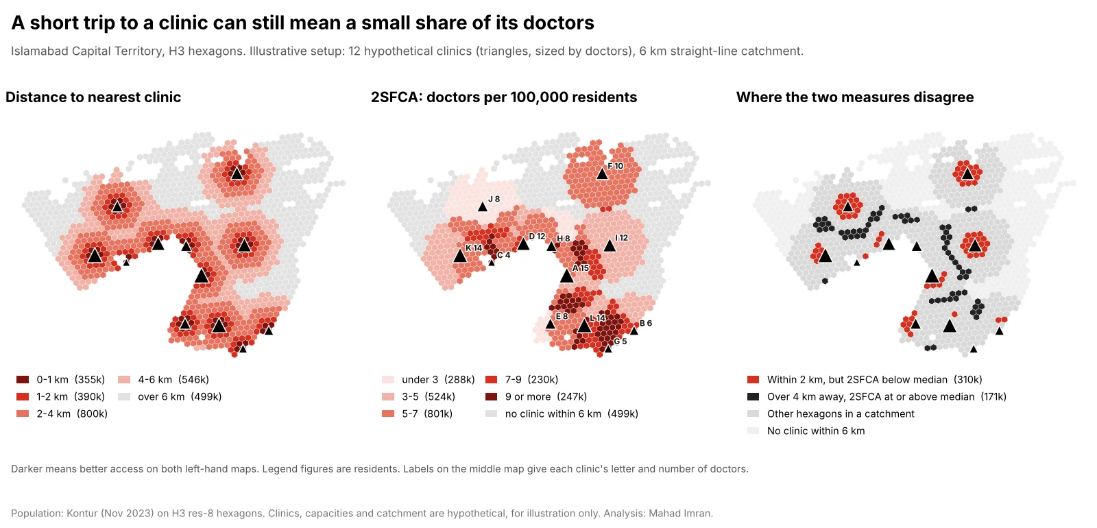
Illustrative setup: 12 hypothetical clinics with 4 to 16 doctors each, 6 km straight-line catchment, Kontur population on H3 resolution-8 hexagons.
The headline numbers:
| Residents | Share | |
|---|---|---|
| Within 1 km of a clinic | 355,283 | 13.7% of all residents |
| Within 2 km of a clinic | 744,960 | 28.8% of all residents |
| Within 2 km, but 2SFCA below the median | 310,413 | 41.7% of those within 2 km |
| More than 4 km away, but 2SFCA at or above the median | 170,779 | 31.3% of covered residents beyond 4 km |
| No clinic within 6 km (2SFCA = 0) | 499,121 | 19.3% of all residents |
Splitting covered residents into fifths on each measure, only 24.7% landed in the same fifth on both, and 43.5% moved by two fifths or more. Of the residents in the closest fifth by distance, 38.7% fell in the bottom two fifths by 2SFCA.
Why the rankings flip
The clinic-level ratios from step 1 explain most of it:
| Clinic | Doctors | Residents within 6 km | Doctors per 100,000 (step 1) |
|---|---|---|---|
| C | 4 | 264,809 | 1.51 |
| H | 8 | 369,124 | 2.17 |
| J | 8 | 334,122 | 2.39 |
| A | 15 | 398,553 | 3.76 |
| F | 10 | 194,586 | 5.14 |
Clinic C sits in a dense area with only 4 doctors, so living next door to it buys little. Clinic F has 10 doctors and fewer than 200,000 people around it. Residents who can reach several clinics add up all of their ratios, so overlap pays. The highest score, 11.9 per 100,000, went to a hexagon 4.2 km from its nearest clinic that falls inside four catchments (C, D, J and K). Across covered hexagons, 2SFCA ranged from 2.2 to 11.9 doctors per 100,000, a fivefold difference that the distance map cannot show. (Summing overlapping catchments this way is one of the known criticisms of 2SFCA, and the three-step variant was designed to temper it.)
What changes with E2SFCA
With distance-decay weights, the picture moves back toward distance. E2SFCA's rank correlation with nearest-clinic distance was -0.81, and its correlation with plain 2SFCA was 0.58. Only 13.9% of residents within 2 km of a clinic scored below the median, against 41.7% under 2SFCA.
The cliff at the catchment edge also softens. The 85,355 residents 5.5 to 6 km from their nearest clinic averaged 4.0 doctors per 100,000 under 2SFCA, close to the city mean, while the 112,552 residents just beyond 6 km scored zero. E2SFCA gave the first group 1.6, which is a more believable step down.
This is a real modelling choice, and the two methods answer slightly different questions. Plain 2SFCA assumes anyone inside the catchment will use any clinic in it. E2SFCA assumes people prefer the nearest. Pick the one that matches how patients behave, and say which you used.
How do you compute 2SFCA in Python?
The core of 2SFCA is a distance matrix and two weighted sums. This is the code behind the Islamabad numbers, using NumPy, pandas and pyproj:
import json
import numpy as np
import pandas as pd
from pyproj import Transformer

def fca2(pop_xy, pop, fac_xy, supply, d0, zones=None):
    """2SFCA, or E2SFCA when zones = [(upper_distance_m, weight), ...]."""
    d = np.hypot(pop_xy[:, None, 0] - fac_xy[None, :, 0],
                 pop_xy[:, None, 1] - fac_xy[None, :, 1])   # metres
    if zones is None:
        w = (d <= d0).astype(float)                     # in the catchment or not
    else:
        w = np.zeros_like(d)
        for upper, weight in sorted(zones, reverse=True):
            w[d <= upper] = weight                      # nearer zones overwrite
    # Step 1: each clinic's doctors divided by the (weighted) population it serves
    demand = (pop[:, None] * w).sum(axis=0)
    ratio = np.divide(supply, demand, out=np.zeros(len(supply)), where=demand > 0)
    # Step 2: each hexagon sums the ratios of every clinic it can reach
    return (w * ratio).sum(axis=1)

hexes = pd.DataFrame(json.load(open("islamabad.json"))["hexes"])
to_utm = Transformer.from_crs(4326, 32643, always_xy=True)     # UTM 43N
x, y = to_utm.transform(hexes.center.str[0].values, hexes.center.str[1].values)
pop_xy, pop = np.column_stack([x, y]), hexes["pop"].to_numpy(float)

# Hypothetical clinics: densest buildable hexagons, at least 4 km apart
sites = []
for i in hexes[hexes.buildable].sort_values("pop", ascending=False).index:
    if all(np.hypot(*(pop_xy[i] - pop_xy[j])) >= 4000 for j in sites):
        sites.append(i)
    if len(sites) == 12:
        break
doctors = np.random.default_rng(2026).integers(4, 17, 12).astype(float)

a2 = fca2(pop_xy, pop, pop_xy[sites], doctors, 6000) * 1e5
ae = fca2(pop_xy, pop, pop_xy[sites], doctors, 6000,
          zones=[(2000, 1.0), (4000, 0.68), (6000, 0.22)]) * 1e5
print((pop * a2).sum() / 1e5, doctors.sum())   # both 116: supply is conserved
For a real study, replace the straight-line matrix d with travel times from a routing engine. An OSRM table request, an ArcGIS Network Analyst origin-destination cost matrix or a pgRouting query all produce the same shape of input. The rest of the function does not change. Walking-based access in Islamabad, computed on the street network, is worked through in the Islamabad school access analysis.
The matrix has one row per population cell and one column per facility, which stays small. Even 100,000 hexagons by 500 clinics is 50 million cells, about 200 MB as 32-bit floats.
What choices change a 2SFCA result the most?
In rough order of impact:
- The catchment size. A larger d0 spreads each clinic's supply over more people and evens out the map. Test at least one shorter and one longer threshold and report how the ranking changes.
- Travel time against straight-line distance. Rivers, ridges, motorways and one-way systems change who can reach what. In Islamabad, the Margalla Hills and the green belts between sectors make straight-line distance especially misleading.
- The capacity measure. Doctors, full-time equivalents, appointment slots and beds give different answers. Use the one that limits service in practice.
- The population layer. 2SFCA divides by population, so errors in the denominator flow straight into the result. Gridded datasets disagree, most of all at the urban edge, and the gridded population comparison shows by how much.
- Edge effects. Clinics just outside the study area serve residents inside it, and residents outside compete for clinics inside. Buffer the study area by at least one catchment width for both supply and demand, then report results only for the core.
- Distance decay. As the Islamabad test showed, moving from 2SFCA to E2SFCA changed the share of near-but-underserved residents from 41.7% to 13.9%.
Which accessibility measure should you use?
Use the simplest measure that answers the question:
- Nearest-facility distance when the issue is travel burden, and capacity is not limiting: post offices, bus stops, pharmacies in a well-supplied city.
- Coverage within a standard for emergency services with a response-time target, ideally as a coverage curve across station counts.
- Cumulative opportunities when choice matters more than crowding, such as jobs or grocery stores reachable in 30 minutes. In the Islamabad test it tracked 2SFCA fairly closely (rank correlation 0.81) because it counts supply, but it cannot tell a crowded clinic from a quiet one.
- 2SFCA or E2SFCA when facilities have finite capacity and people compete for it: primary care, hospital beds, school places, childcare. Prefer E2SFCA when people mostly use the nearest facility, and report the plain 2SFCA alongside it if the choice is contested.
What should you take from this?
Distance to the nearest clinic measures how far people travel. Whether a doctor is free when they arrive depends on capacity and competing demand, and 2SFCA adds both with very little extra computation. In the Islamabad test, that changed the ranking for most residents and flagged hundreds of thousands of people who live close to a clinic that is badly overstretched. Use network travel times, state the catchment and the capacity measure, test the sensitivity, and map the ratio next to the distance so readers can see where the two disagree.
If you need a healthcare, school or service accessibility study built on real facility and population data, email me at mahad.imran29@gmail.com.