A coverage curve shows how many people a given number of stations can reach within a response-time standard, when each count is placed as well as possible. In three cities tested at a 12-minute drive, the first few stations reached most residents and the curve then flattened fast. Calgary reached 96% with 6 stations, but covering every reachable resident took 39.
This article shows how to build that curve, what the three test cities say about it, why adding stations one at a time does worse than planning them together, and how to use the curve when a council asks how many stations it actually needs.
What is a coverage curve?
A coverage curve plots two things against each other:
- Horizontal axis: the number of stations, depots or facilities.
- Vertical axis: the best coverage that many stations can achieve, usually the share of residents or historical incidents within a response-time standard.
Each point on the curve is its own optimization. The point at 4 stations is the best possible placement of 4 stations, found from scratch, and it does not have to share any sites with the best placement of 3.
The model behind each point is the maximal covering location problem (MCLP), introduced by Church and ReVelle in 1974. It fixes the number of facilities and places them to cover as much demand as possible within a distance or time standard. Its partner, the location set covering problem, asks the reverse question: the fewest facilities needed to cover all demand. Both are explained in more depth, with a worked Calgary example at the NFPA 4-minute standard, in fire station location analysis.
The curve matters because neither single answer is what a decision maker needs. "4 stations cover 84%" and "39 stations cover everyone" are both true. The useful information is the shape between them.
How was this test set up?
I used the three cities behind the Site Selection Showdown game on this site, which share one method:
- Population: Kontur Population on H3 hexagons at resolution 8, each about 0.7 km², clipped to each city's OpenStreetMap boundary.
- Road network: the OpenStreetMap drive network, with one speed per road class, calibrated per city against the OSRM routing engine. These are free-flow times with no congestion.
- Candidate sites: hexagons with a drivable road that are not mostly park, water, forest or airfield. That leaves 1,114 candidates in Calgary, 906 in Islamabad and 308 in Bahawalpur.
- Standard: a 12-minute drive from the station to the centre of each hexagon. This is looser than the urban fire standards, and it is in the range planners use for EMS and for rural or suburban fire service. It keeps the curves readable for cities of different sizes.
- Solver: each point is an exact integer program solved with CBC through PuLP, not a heuristic. The 3-station result for Calgary matches the optimum published in the game (1,007,984 residents), which is a useful check.
| City | Modelled population | Area | Hexagons | Candidate sites |
|---|---|---|---|---|
| Calgary | 1,463,328 | 853 km² | 1,205 | 1,114 |
| Islamabad Capital Territory | 2,590,233 | 963 km² | 1,164 | 906 |
| Bahawalpur | 673,192 | 399 km² | 542 | 308 |
What do the coverage curves look like?
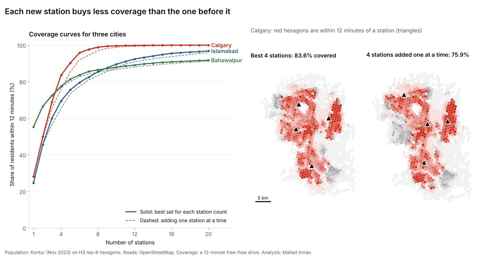
Solid lines: the best placement for each station count. Dashed lines: stations added one at a time, each the best addition given the ones already built.
| Stations | Calgary | Islamabad | Bahawalpur |
|---|---|---|---|
| 1 | 28.1% | 24.7% | 55.3% |
| 2 | 49.8% | 45.5% | 66.5% |
| 3 | 68.9% | 60.0% | 72.5% |
| 4 | 83.6% | 69.5% | 77.6% |
| 5 | 90.3% | 75.5% | 81.4% |
| 6 | 95.8% | 79.6% | 83.6% |
| 7 | 97.6% | 82.5% | 85.6% |
| 8 | 98.9% | 85.4% | 86.4% |
| 10 | 99.6% | 89.6% | 87.9% |
| 15 | 99.9% | 94.9% | 90.6% |
| 20 | 100.0% | 96.8% | 91.7% |
Bold marks the first count to pass 80%.
The marginal station
The curve is easier to argue about as the number of new residents each extra station adds:
| Station number | Calgary adds | Islamabad adds | Bahawalpur adds |
|---|---|---|---|
| 1st | 411,570 | 638,574 | 372,551 |
| 2nd | 317,565 | 540,014 | 75,307 |
| 3rd | 278,849 | 375,446 | 39,920 |
| 4th | 215,212 | 245,705 | 34,386 |
| 5th | 98,052 | 156,378 | 25,797 |
| 6th | 81,212 | 105,330 | 15,128 |
| 7th | 26,184 | 76,008 | 13,050 |
| 8th | 18,364 | 74,526 | 5,796 |
| 9th | 7,721 | 58,154 | 5,214 |
| 10th | 2,807 | 49,625 | 4,469 |
In Calgary the 10th station adds less than 1% of what the 1st did. The operating cost of a staffed station does not fall in the same way: a crew costs the same whether it protects 400,000 people or 3,000. That gap is the whole argument for drawing the curve.
What it takes to reach everyone
| Calgary | Islamabad | Bahawalpur | |
|---|---|---|---|
| Stations for 80% | 4 | 7 | 5 |
| Stations for 90% | 5 | 11 | 14 |
| Stations for 95% | 6 | 16 | not reachable |
| Share of residents any candidate can reach | 99.99% | 99.55% | 93.17% |
| Stations to cover every reachable resident | 39 | 54 | 42 |
The last row is the location set covering answer. Going from 95% to everyone took Calgary 33 more stations. Islamabad needed 38 more after its 16th. These final stations protect a few hundred to a few thousand people each, scattered on the urban edge.
Why are the three curves so different?
The shape comes from where people live relative to the road network, not from population alone.
- Bahawalpur starts high and stalls. One well-placed station reaches 55% of the city because the old city and its surrounding neighbourhoods are compact. But 6.8% of the modelled population lives in hexagons that no candidate site can reach within 12 minutes, so the curve can never pass 93.2%. Those 45,996 people live in 110 hexagons whose median distance from the city's population centre is 14 km, on the rural fringe inside the boundary, where the road network is sparse.
- Calgary climbs fastest after the first station. Its population is spread out, so one station only reaches 28%, but the freeway ring and arterial grid let each new station claim a large, distinct catchment. By 6 stations the curve is nearly flat.
- Islamabad climbs slowly for longest. The capital territory is split by the Margalla Hills, Rawal Lake and large green belts, and its population is spread across separate clusters: the planned sectors, the housing schemes to the south and east, and the villages beyond. Each station covers a smaller share, and the curve keeps adding about 50,000 or more residents per station out to the 10th.
The lesson for a client: never borrow another city's number. A rule of thumb such as "one station per 50,000 residents" would give about 29 stations for Calgary, 52 for Islamabad and 13 for Bahawalpur. None of those counts sits at a meaningful point on the curves above.
Is adding one station at a time good enough?
Most real networks grow one station at a time, so it is tempting to plan them that way: pick the best first site, then the best second site given the first, and so on. This is a greedy approach, and it is what happens by default when each new station is justified on its own.
It costs coverage. The dashed lines in the figure show the gap:
| Stations | Calgary, planned together | Calgary, one at a time | Residents lost |
|---|---|---|---|
| 3 | 1,007,984 | 958,268 | 49,716 |
| 4 | 1,223,196 | 1,110,101 | 113,095 |
| 5 | 1,321,248 | 1,250,445 | 70,803 |
| 6 | 1,402,460 | 1,345,717 | 56,743 |
At four stations, the one-at-a-time network covers 7.7 percentage points fewer Calgarians. Islamabad loses up to 107,252 residents (4.1 points) at four stations. Bahawalpur's loss is smaller, at most 1.5 points, because its curve is dominated by one central site.
The reason is that the best first station is usually a compromise placed in the middle of everything. Once more stations exist, that central position is wasted, because its catchment overlaps with all of them. In Calgary the best set of three stations and the best set of four share only one site. A plan that locked in the first three would never reach the best four.
What this means in practice:
- Plan the target network first, for the station count you expect in 10 to 20 years, then decide the build order.
- Build toward it. Choose the first stations from the long-term set, ordered by how much each covers on its own. That gives up a little coverage early to avoid a permanent loss later.
- Re-solve when the city changes. A new freeway interchange or a large subdivision can move the optimal set. Rerun the curve with existing stations fixed in place, which an integer program handles with one extra constraint per station.
How do you use the curve in a decision?
The curve does not choose a number for you. It shows the trade-off so the decision can be made on purpose.
- Fix the standard first. Career fire departments in the US often plan to the 240-second first-engine travel time in NFPA 1710. Volunteer and combination departments use NFPA 1720, which sets 9 minutes for urban demand zones (over 1,000 people per square mile), 10 for suburban and 14 for rural. In Punjab, Rescue 1122 reports a provincial average response time of about 7 minutes. A curve at the wrong standard answers the wrong question.
- Draw the curve for that standard, and for one stricter and one looser standard. If the recommended count changes a lot between them, the standard is the real decision, not the count.
- Put a cost on the vertical axis. Divide each station's annual operating cost by the residents or incidents it adds. Where that number crosses what the community is willing to pay per person covered, you have a defensible count.
- Name the people left out. The flat end of the curve is not empty. It is specific neighbourhoods. Map them and decide whether they get a station, a mutual-aid agreement with a neighbouring service, a rapid-response vehicle, or a lower standard written into policy.
- Use incidents if you have them. Population is a proxy for demand. Historical call locations, weighted by severity, are better, and they usually make the curve rise faster because calls cluster more tightly than homes.
What are the limitations of this test?
- Free-flow speeds. Travel times come from road-class speeds calibrated to OSRM, which has no congestion. Peak-hour curves would sit lower and flatten later.
- Modelled population. Kontur is a modelled grid, not a census count, and residents just outside each boundary are ignored, as are stations in neighbouring jurisdictions that could serve the edge.
- Population, not incidents. Every resident counts equally. Real demand is uneven across age, land use and time of day.
- One crew per station, always available. Coverage models assume a station's crew is free when a call comes in. In busy systems they often are not. Backup-coverage and probabilistic models handle that, and they push the recommended count up.
- A 12-minute standard. At 4 or 8 minutes every curve would rise more slowly and need many more stations. The shape, steep then flat, holds at any standard. The numbers do not.
What should you take from this?
If you are asked how many stations a city needs, answer with a curve, not a number. Solve the best placement for every count from one to well past the current network, mark where the next station adds too few people to justify its cost, and plan the whole network before deciding the order to build it in. Then show the map of who is still outside the line, because that is what the council will be asked about.
If you want a coverage curve and a station plan built for your service area, email me at mahad.imran29@gmail.com.