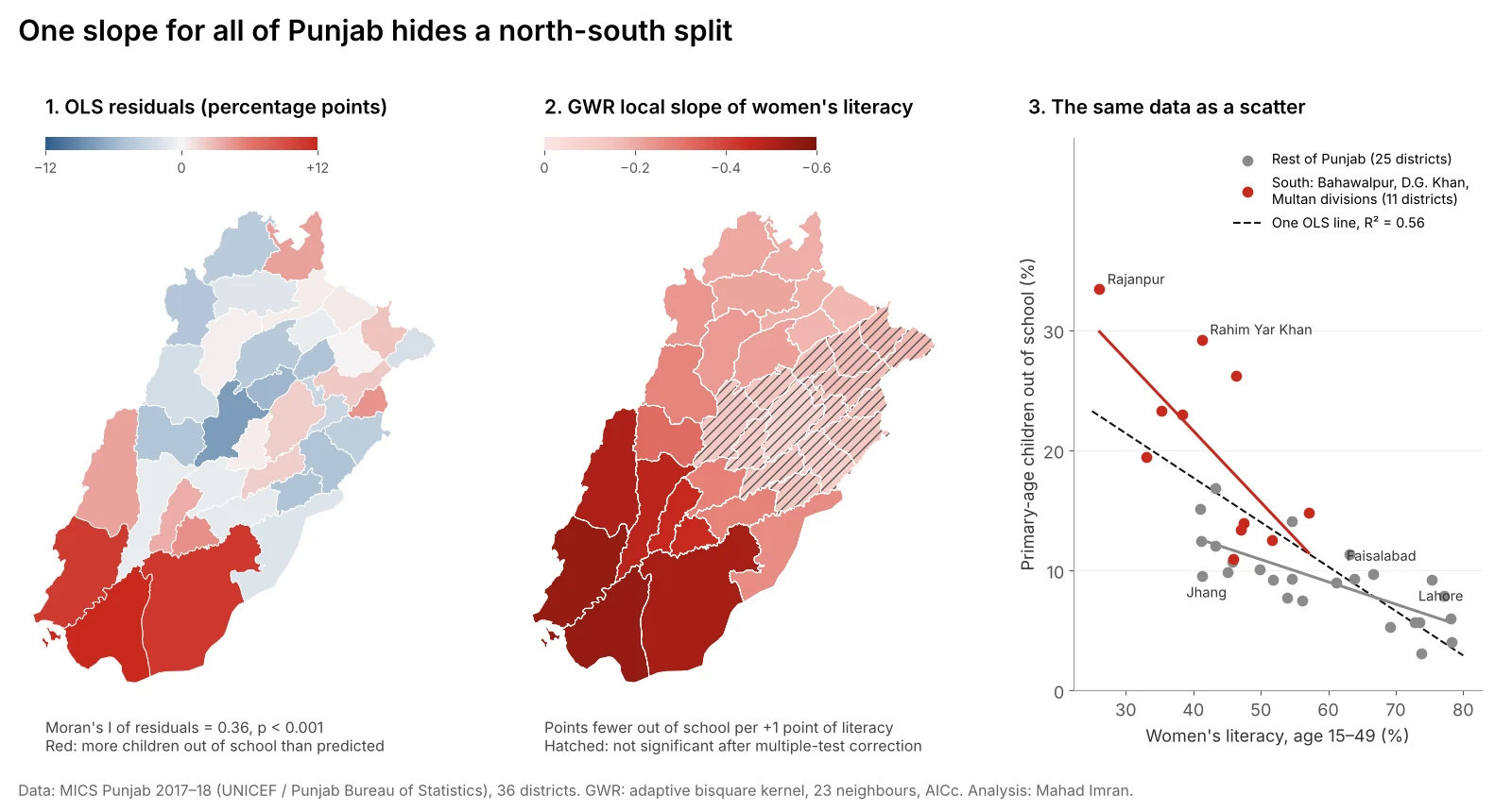
Geographically weighted regression (GWR) fits a separate regression around every location, so a coefficient can change across a map. On Punjab's 36 districts, an ordinary regression of children out of school on women's literacy explained 56% of the variation but left its errors clustered in the south (Moran's I = 0.36). GWR raised R² to 0.84 and showed why: in the southern districts the slope was about three times steeper than around Faisalabad and Lahore.
This article walks through that test from start to finish: the global model, the residual check that says something spatial is missing, the GWR fit, how to read its maps without fooling yourself, and the simpler model that GWR pointed to.
What problem does GWR solve?
A standard regression, ordinary least squares (OLS), estimates one coefficient per predictor for the whole study area. That is a strong assumption. It says the effect of a predictor is the same in Rajanpur as in Rawalpindi.
When that assumption fails, two things go wrong:
- The coefficient becomes an average of different local relationships, and may describe no place well.
- The errors cluster in space. Districts where the true effect is stronger sit together on the map, and all of them get under-predicted together.
GWR, introduced by Brunsdon, Fotheringham and Charlton (1996), drops the assumption. For each location it fits a weighted regression in which nearby observations count more than distant ones. The output is a coefficient for every location, which you can map.
What data did I use?
The example uses district data that also sits behind this site's Punjab education map:
- Outcome: the share of primary-age children out of school, from MICS Punjab 2017–18, the Multiple Indicator Cluster Survey run by the Punjab Bureau of Statistics with UNICEF. It ranges from 3.1% in Narowal to 33.4% in Rajanpur.
- Predictor: the literacy rate of women aged 15 to 49 from the same survey, a common proxy for mothers' education. It ranges from 26.1% in Rajanpur to 78.3% in Gujrat.
- Units: Punjab's 36 districts.
I kept to one predictor on purpose. With 36 observations, each local regression only has a couple of dozen neighbours to learn from, and one predictor keeps the method visible. The same district data was used for hot spot analysis with Moran's I and Getis-Ord Gi*, which is a good primer on the spatial statistics used below.
Step 1: Fit the global model
The OLS model is simple and, on its face, convincing:
| Term | Coefficient | Std. error | t | p |
|---|---|---|---|---|
| Intercept | 32.50 | 3.16 | 10.30 | < 0.001 |
| Women's literacy (%) | −0.370 | 0.057 | −6.55 | < 0.001 |
R² = 0.56. Each 10-point rise in women's literacy goes with about 3.7 fewer percentage points of children out of school. Most reports would stop here.
Step 2: Check the residuals for spatial autocorrelation
Before trusting any regression on map data, map its residuals and test them. I used Queen contiguity weights, where districts that share a border are neighbours, and a permutation test with 9,999 draws.
Moran's I of the OLS residuals = 0.36, p < 0.001.
That is strong clustering. The three largest positive residuals, meaning more children out of school than literacy predicts, were all in the far south: Rahim Yar Khan (+12.0 points), Bahawalpur (+10.9) and Rajanpur (+10.6). The largest negative residuals were in the centre: Jhang (−7.7) and Chiniot (−6.0). The left map in the figure below shows the pattern.
Clustered residuals mean three things for the OLS model. Its standard errors are too small, so the p-value overstates certainty. Its single coefficient is an average across regions that behave differently. And there is a spatial process the model has not captured.
Step 3: Fit GWR
GWR needs two choices: a kernel, which sets how weight falls off with distance, and a bandwidth, which sets how far it reaches.
- Kernel: adaptive bisquare. "Adaptive" means the bandwidth is a number of neighbours, not a fixed distance, which suits districts of very different sizes.
- Bandwidth: chosen by minimising AICc, a criterion that rewards fit and penalises complexity. The search settled on 23 nearest neighbours, so each district's regression leans on roughly two thirds of the province, with the closest districts weighted most.
| Model | R² | Adj. R² | AICc | Residual Moran's I |
|---|---|---|---|---|
| OLS | 0.56 | 0.55 | 216.4 | 0.36 (p < 0.001) |
| GWR (bw = 23) | 0.84 | 0.80 | 196.8 | 0.10 (p = 0.12) |
GWR used the equivalent of 6.8 parameters instead of 2 and still came out about 20 AICc points better, a large margin. Its residuals are no longer significantly clustered. A Monte Carlo test of whether the literacy coefficient really varies across space, in which the district locations are reshuffled and the model refitted, gave p < 0.02.
Step 4: Read the coefficient map
The local slope for women's literacy ranged from −0.55 to −0.07:
| District | Division | Local slope | Significant? |
|---|---|---|---|
| Rahim Yar Khan | Bahawalpur | −0.55 | Yes |
| Rajanpur | Dera Ghazi Khan | −0.55 | Yes |
| Bahawalpur | Bahawalpur | −0.52 | Yes |
| Multan | Multan | −0.45 | Yes |
| Rawalpindi | Rawalpindi | −0.19 | Yes |
| Lahore | Lahore | −0.15 | No |
| Jhang | Faisalabad | −0.12 | No |
| Faisalabad | Faisalabad | −0.07 | No |
Averaged by division, the slope was −0.46 in Dera Ghazi Khan and −0.44 in Bahawalpur, against −0.11 in Faisalabad and Sahiwal. In plain words: in the south, a 10-point gain in women's literacy goes with about 5 fewer points of children out of school. In central Punjab it goes with about 1.
Significance needs care. GWR runs one test per location, 36 here, and the tests overlap because neighbouring regressions share data. A plain 5% threshold would flag too many. I used the correction of da Silva and Fotheringham (2016), built into mgwr as filter_tvals(). After it, the slope was significant in 21 of 36 districts. The 15 that were not, hatched in the middle map, form one block in central and north-eastern Punjab.
Is the variation really spatial, or just a curve?
This is the question I would ask of any GWR result, and it often goes unasked. If the true relationship is curved, flattening out as literacy rises, then low-literacy districts will show steep slopes and high-literacy districts flat ones. Because low-literacy districts cluster in the south, GWR will paint that curve as a spatial pattern.
So I tested non-spatial alternatives:
| Model | Parameters | R² | Residual Moran's I |
|---|---|---|---|
| OLS, straight line | 2 | 0.56 | 0.36 (p < 0.001) |
| OLS with a quadratic term | 3 | 0.64 | 0.25 (p = 0.007) |
| OLS on log of out-of-school rate | 2 | 0.62 | 0.35 (p = 0.001) |
| OLS with a south indicator and interaction | 4 | 0.76 | 0.01 (p = 0.34) |
| GWR | 6.8 effective | 0.84 | 0.10 (p = 0.12) |
A curve helps a little but leaves the residuals clustered. A simple regional split does almost all the work. With an indicator for the three southern divisions (Bahawalpur, Dera Ghazi Khan and Multan, 11 districts) and its interaction with literacy, the slope is −0.59 in the south and −0.19 elsewhere, and the residual clustering disappears.
That is how I would use GWR in practice: as a diagnostic that finds where a relationship changes, followed by a simpler, explainable model that names the change. The likely reasons behind the southern pattern, such as poverty, distance to the nearest girls' school, and seasonal farm work in the cotton belt, are what the next model should measure directly.
How do you run GWR in Python?
The mgwr package from PySAL does bandwidth selection, fitting, inference and multiscale GWR:
import geopandas as gpd
import numpy as np
from libpysal.weights import Queen
from esda.moran import Moran
from mgwr.sel_bw import Sel_BW
from mgwr.gwr import GWR
import statsmodels.api as sm

g = gpd.read_file("punjab_districts.gpkg").to_crs(32643)  # projected, metres
y = g[["oos_primary"]].values
X = g[["lit_women"]].values

# 1. Global model and residual check
ols = sm.OLS(y, sm.add_constant(X)).fit()
w = Queen.from_dataframe(g); w.transform = "r"
print(Moran(ols.resid, w, permutations=9999).I)

# 2. Bandwidth by AICc, then GWR
coords = np.c_[g.centroid.x, g.centroid.y]
bw = Sel_BW(coords, y, X, kernel="bisquare", fixed=False).search(
    criterion="AICc", bw_min=8, bw_max=len(g))
res = GWR(coords, y, X, bw, kernel="bisquare", fixed=False).fit()

g["slope"] = res.params[:, 1]
g["slope_sig"] = res.filter_tvals()[:, 1] != 0   # corrected for multiple tests
g["local_r2"] = res.localR2.ravel()
print(bw, res.R2, res.aicc)
Three practical notes:
- Cap the bandwidth search at the number of observations when the dataset is small. Without
bw_max, the default search range can ask for more neighbours than exist. - Use projected coordinates in metres, or pass
spherical=Truewith longitude and latitude. At Punjab's latitudes a degree of longitude is about 14% shorter on the ground than a degree of latitude, so distances in raw degrees distort every neighbourhood. - Report the corrected significance, not the raw t-values. Maps of raw local p-values look convincing and are mostly noise.
When is GWR the wrong tool?
- Too few observations for the number of predictors. Local estimates become unstable and the coefficient maps show patterns that are not there. Keep to one or two predictors with a few dozen units.
- Correlated predictors. Local multicollinearity is worse than global multicollinearity because each local sample is small. Check local condition numbers, which
mgwrreports, and drop or combine predictors when they run high. - Prediction outside the data. GWR describes the places you fitted. It is not a forecasting model for new areas.
- When predictors act at different scales. One bandwidth for all coefficients is a strong assumption. Multiscale GWR (MGWR) gives each coefficient its own bandwidth and is usually the better default once you have several predictors and a few hundred observations.
- When the real issue is spillover. If one district's outcome is driven by its neighbours' outcomes, a spatial lag or spatial error model, available in PySAL's
spreg, is the right family, not GWR.
What are the limits of this example?
- 36 districts is small. The result is exploratory, and a bandwidth of 23 means each local model shares most of its data with its neighbours.
- One survey round. MICS 2017–18 is now several years old and the out-of-school rates have sampling error of their own, which is larger in smaller districts.
- Ecological data. These are district averages. They say nothing about whether a given literate mother's children attend school, and reading them that way is the ecological fallacy. The same district pattern can also shift when units are drawn differently, a problem covered in the modifiable areal unit problem.
What should you take from this?
Always map the residuals of a regression on spatial data and test them with Moran's I. If they cluster, a single coefficient is hiding something. GWR is a quick, honest way to see what: where the relationship is strong, where it fades, and whether the difference survives a correction for multiple tests. Then use what it shows to build a simpler model you can explain to a ministry or a client, with the regional difference written into it.
If you need a regression or targeting analysis on district, tract or customer data that accounts for where things are, email me at mahad.imran29@gmail.com.