A weighted overlay scores every candidate location by putting each criterion on a common scale, multiplying it by a weight and adding the results. The analytic hierarchy process (AHP) is the most common way to set those weights defensibly. In a test on 1,114 candidate sites in Calgary, small changes to AHP weights barely moved the top 10, but two quieter choices, how criteria were scaled and whether AHP was used at all, replaced up to 7 of them. And because the method scores sites one at a time, its 10 best sites all sat within 3.5 km of each other.
Weighted overlay, also called suitability analysis or GIS multi-criteria decision analysis (MCDA), is often the first tool reached for in site selection. It is easy to explain and fast to run. This article shows how to set the weights properly, how to test whether they matter, and the one situation where the method gives a misleading answer.
What is weighted overlay?
Weighted overlay answers the question "how suitable is each location?" in four steps:
- Choose criteria that matter to the decision: demand, access, cost, constraints.
- Standardise each criterion onto a common scale, such as 0 to 1, so that residents and kilometres can be added together.
- Weight each criterion by its importance, with weights that sum to 1.
- Sum the weighted values for every cell or candidate site, and rank.
Hard constraints, such as flood zones, protected land or sites that cannot be zoned, are applied as masks before scoring, not as low weights. A site in a floodway should be excluded, not merely marked down. Malczewski's (2006) review of more than 300 GIS-MCDA journal articles published between 1990 and 2004 found simple weighted summation and Boolean overlay to be the most common ways of combining criteria.
How do you set the weights with AHP?
The analytic hierarchy process, developed by Thomas Saaty in the 1970s, replaces "pick some percentages" with a series of two-way comparisons that are easier to judge. For each pair of criteria, the decision maker answers: how much more important is A than B, on a scale where 1 means equal, 3 moderately more, 5 strongly more, 7 very strongly more and 9 extremely more?
A worked example: the next clinic in Calgary
To make this concrete, I set up a realistic problem on the Site Selection Showdown data for Calgary. A clinic operator has three existing clinics, placed at the three sites that together reach the most residents within a 12-minute drive. Those three reach 68.9% of the city's 1.46 million modelled residents. The operator wants to rank the 1,114 buildable candidate sites for the next clinic, using three criteria:
| Criterion | What it measures | Range across sites |
|---|---|---|
| Unserved demand | Residents within 12 minutes who are not within 12 minutes of an existing clinic | 0 to 196,382 |
| Total reach | All residents within a 12-minute drive | 5 to 411,570 |
| Local density | Residents in the site's H3 hexagon and its 6 neighbours, a walk-in catchment of about 5 km² | 3 to 44,672 |
The operator's judgements, written as a pairwise comparison matrix:
| Unserved | Reach | Local | |
|---|---|---|---|
| Unserved | 1 | 3 | 5 |
| Reach | 1/3 | 1 | 2 |
| Local | 1/5 | 1/2 | 1 |
The weights are the principal eigenvector of this matrix, normalised to sum to 1:
| Criterion | AHP weight |
|---|---|
| Unserved demand | 0.648 |
| Total reach | 0.230 |
| Local density | 0.122 |
Check the consistency ratio
AHP also tells you whether the judgements hang together. If A is 3 times B and B is 2 times C, then A should be about 6 times C. The consistency ratio (CR) measures how far the matrix departs from that ideal, compared with random judgements. Saaty's threshold is CR < 0.10.
Here CR = 0.003, comfortably consistent. With four or more criteria, it is common to get a CR above 0.10 on the first try. When that happens, show the decision makers which comparison is out of line and ask them to reconsider it, rather than adjusting the numbers yourself.
import numpy as np

A = np.array([[1, 3, 5],
              [1/3, 1, 2],
              [1/5, 1/2, 1]])

vals, vecs = np.linalg.eig(A)
k = np.argmax(vals.real)
w = np.abs(vecs[:, k].real); w /= w.sum()          # weights

n = A.shape[0]
RI = {3: 0.58, 4: 0.90, 5: 1.12, 6: 1.24, 7: 1.32}[n]  # Saaty's random index
CR = ((vals.real[k] - n) / (n - 1)) / RI
print(w.round(3), round(CR, 3))   # [0.648 0.23 0.122] 0.003
How sensitive is the result to the weights?
Weights come from judgement, so the honest question is whether different but reasonable judgements would change the answer. I tested three kinds of change against the baseline top 10.
1. Moving one weight at a time
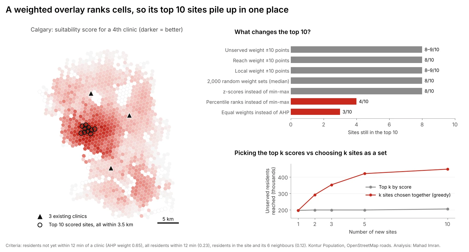
Adding or removing 10 percentage points from one weight, and rescaling the others proportionally, kept 8 or 9 of the top 10 sites in every case. The top-ranked site never changed.
2. Thousands of plausible weight sets
To test many judgements at once, I drew 2,000 weight sets from a Dirichlet distribution centred on the AHP weights. In 90% of draws the unserved weight fell between 0.47 and 0.81, reach between 0.09 and 0.40, and local density between 0.03 and 0.26, a wide spread of opinion.
| Result across 2,000 weight sets | Value |
|---|---|
| Median number of baseline top-10 sites kept | 8 |
| Draws keeping 8 or more | 81% |
| Draws keeping 5 or fewer | 6% |
| Different sites that ever appeared in a top 10 | 32 |
| Draws where the baseline #1 site stayed #1 | 95.5% |
This is the most useful output of the whole exercise. It splits the candidates into a core that wins under almost any reasonable weighting and a fringe whose rank depends on whose opinion counts. Present both to the decision makers.
3. Design choices that look technical
Two choices that rarely get discussed moved the result far more than the weights did:
| Change | Top-10 sites kept | Same #1? |
|---|---|---|
| Z-scores instead of min-max scaling | 8 | Yes |
| Percentile ranks instead of min-max scaling | 4 | No |
| Equal weights instead of AHP | 3 | No |
Scaling changes the effective weights. Min-max scaling stretches each criterion from its minimum to its maximum, so a criterion with one extreme outlier gets compressed for every other site. Percentile ranks spread every criterion evenly, which gives small differences in the middle of the range as much influence as large ones at the top. Neither is wrong, but they encode different views, so pick one deliberately and say which.
Equal weights are often used as a "neutral" default. They are a strong claim that local walk-in density matters as much as unserved demand. Here that claim replaced 7 of the top 10 sites.
What is the clustering trap?
The map in the figure shows the more serious problem. The 10 highest-scoring sites all sit within 3.5 km of each other, with a median distance of 1.6 km between them. They share almost the same catchment.
That is not a quirk of this example. Weighted overlay scores each location on its own merits, so neighbouring cells with similar surroundings get similar scores, and the top of the list is a single hot spot seen ten times. The method has no idea that opening site #1 makes site #2 much less useful.
The cost is large when you need more than one site:
| New sites | Top k by score: unserved residents reached | k sites chosen together | Difference |
|---|---|---|---|
| 1 | 196,382 | 196,382 | 0% |
| 2 | 198,716 | 291,654 | +47% |
| 3 | 198,716 | 352,081 | +77% |
| 5 | 198,716 | 420,296 | +112% |
| 10 | 204,911 | 447,347 | +118% |
The "chosen together" column adds sites one at a time, each time picking the site that reaches the most residents not yet covered by the others. That is a simple greedy version of the maximal covering problem. An exact solver would do slightly better still, as shown in how many stations is enough. Ten sites chosen that way reach 98% of the 455,344 unserved residents. Ten sites taken from the top of the suitability list reach 45%.
Rule of thumb: use weighted overlay to screen and rank sites for one decision at a time, or to remove poor areas before modelling. When the question is "where should our next three locations go?", switch to a location-allocation model that chooses them as a set. The fire station location analysis article explains those models, and retail and franchise site selection with GIS shows how cannibalization between stores is handled.
A checklist for a weighted overlay you can defend
- Separate constraints from criteria. Mask out what is impossible before scoring.
- Check for double counting. Here, total reach and local density correlate at 0.59, because dense places also have more people within 12 minutes. Two correlated criteria quietly give that idea more weight than the AHP says.
- Choose and state the scaling method. Min-max, z-score or rank, and why.
- Set weights with stakeholders using AHP, and keep the consistency ratio below 0.10.
- Run a weight sensitivity test, one-at-a-time and Monte Carlo, and report which sites are stable.
- Do not take the top k for k sites. Use the scores to shortlist, then choose the set with a coverage or allocation model.
- Visit the shortlist. Scores built from population and roads miss lease terms, visibility, parking and access from the right side of a divided road.
What are the limits of this test?
- A stylised problem. Real clinic siting would add land cost, competitors, zoning and patient mix. More criteria usually mean more sensitivity, not less.
- Modelled population and free-flow travel times. Both come from the same Kontur and OpenStreetMap data as the Site Selection game, with no congestion.
- Existing clinics are hypothetical. I placed them at the best three-site solution so the unserved criterion has a clear meaning.
- Greedy, not optimal, sets. The set results are a lower bound on what an exact model would find.
What should you take from this?
Weighted overlay with AHP weights is a sound way to rank locations, as long as you test it. Small changes in weights rarely matter much. The choices around them, how criteria are scaled, whether they overlap, and whether you rank sites individually or choose them as a group, often matter more. Report the stable core of sites, not one ranked list, and never pick several sites off the top of a suitability map.
If you need a site suitability or network expansion study that will stand up in front of a board or council, email me at mahad.imran29@gmail.com.