Sentinel-2 imagery is delivered as tiles of 10,980 by 10,980 pixels at 10 m, or 109.8 km on a side, laid out on a 100 km step of the Military Grid Reference System (MGRS). Each tile is projected in its own UTM zone, and neighbouring tiles in a zone overlap by about 9.8 km. Punjab, Pakistan needs 39 tiles, 20 in zone 42N and 19 in zone 43N, so a provincial mosaic has to be reprojected onto one grid before any tiles are combined.
This article explains how the tile grid and its names work, how much the tiles overlap, which target CRS and resampling to choose, how to resolve overlaps and level scenes from different dates, and how the 2022 processing baseline change affects mosaics. It ends with code for STAC search, rasterio and GDAL.
What is the Sentinel-2 tile grid?
The Sentinel-2 tile grid is a fixed set of square tiles defined in UTM on the WGS 84 datum, one family per UTM zone, named after the MGRS 100 km squares they sit on. ESA describes it as a 100 km step with tiles enlarged to give a large overlap with their neighbours. The grid file ESA publishes contains 56,686 tiles; I used a GeoParquet conversion of it for every count in this article.
A tile ID such as 43RCN reads as:
- 43: the UTM zone, here 72°E to 78°E (EPSG:32643 on WGS 84).
- R: the 8-degree MGRS latitude band, here 24°N to 32°N. The next band north, S, starts at 32°N, which is why Punjab's tiles carry both R and S.
- CN: the 100 km square within that zone.
Product names carry the ID with a T prefix, as in S2B_MSIL2A_..._T43RCN_....
| Band resolution | Pixels per tile side | Bands |
|---|---|---|
| 10 m | 10,980 | B02, B03, B04, B08 |
| 20 m | 5,490 | B05, B06, B07, B8A, B11, B12, SCL |
| 60 m | 1,830 | B01, B09, B10 (L1C) |
The tile corners sit just off round numbers. The upper-left eastings of Punjab's tiles are 199,980, 300,000, 399,960, 499,980, 600,000 and 699,960 m, so the step alternates between 100,020 and 99,960 m and the overlap between neighbours in a zone is 9.78 to 9.84 km.
How do Sentinel-2 tiles overlap at a UTM zone boundary?
At a zone boundary the overlap is much wider, because each zone's tiles run past the boundary meridian into the next zone. Along 72°E, the zone 42N tiles extend east to between 72.15°E and 72.33°E across Punjab, and the zone 43N tiles extend west to between 71.95°E and 71.77°E. The strip imaged in both zones is about 20 km wide at 28°N, 31 km at 30°N, 43 km at 32°N and 52 km at 33.5°N.
I intersected the official tile footprints with Punjab's outline, the union of the 36 district boundaries used in my Punjab education map, and sampled the province on a 0.01° grid weighted by area:
| Coverage of Punjab | Share of area |
|---|---|
| Imaged by exactly 1 tile | 73.4% |
| Imaged by 2 tiles | 24.7% |
| Imaged by 3 or 4 tiles (corners) | 1.9% |
| Imaged by tiles from both UTM zones | 10.8% |
So every acquisition over a quarter of the province arrives at least twice, and over a tenth of it arrives twice in two different coordinate systems.
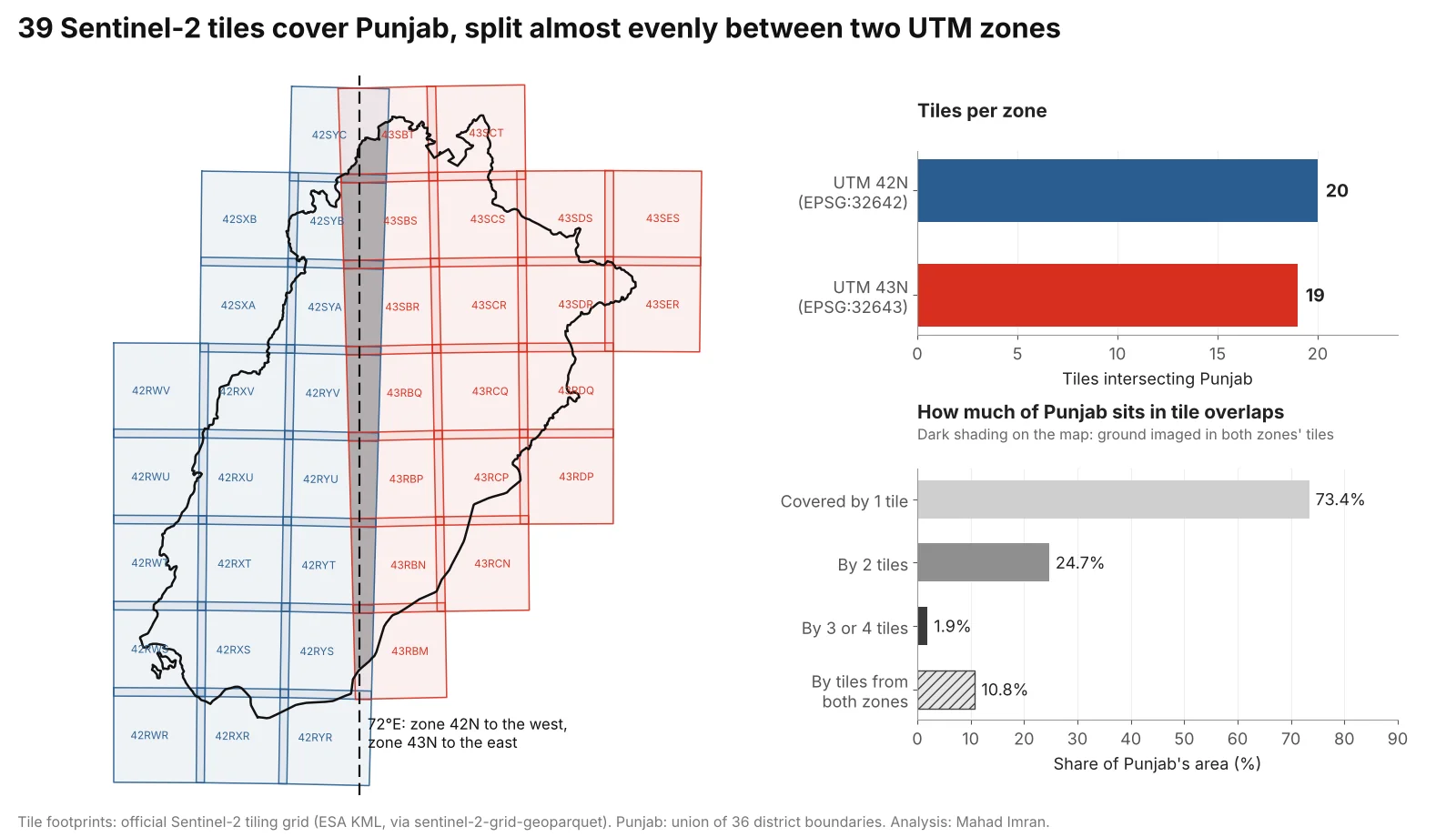
Each tile is 109.8 km square in its own zone, so the two families meet at an angle of about 3° along 72°E.
Why can't you mosaic tiles from different UTM zones directly?
Tiles from different zones use different coordinate systems, so their pixel grids do not line up. The same easting and northing in EPSG:32642 and EPSG:32643 are hundreds of kilometres apart on the ground, and the two grids are rotated against each other by the difference in meridian convergence: 2.8° at 28°N and 3.4° at 34°N along 72°E. No shift or crop can align them. Every pixel from at least one zone has to be resampled.
Tools signal this in different ways. gdalbuildvrt skips inputs whose projection differs from the first file, with a warning. Merge functions that assume a shared CRS can silently produce nonsense. The safe pattern is always the same: pick one target CRS and one target grid, then warp every tile onto it.
Which target CRS should a cross-zone mosaic use?
For a provincial mosaic, use the UTM zone that holds most of the area, or a custom transverse Mercator centred on the area if scale error matters. I calculated the scale factor at every point of a 0.05° grid inside Punjab with pyproj:
| Target CRS | Scale error across Punjab | Notes |
|---|---|---|
| WGS 84 / UTM 43N (EPSG:32643) | −0.04% to +0.34% | Worst at the western edge; eastings go negative west of roughly 69.8°E |
| WGS 84 / UTM 42N (EPSG:32642) | −0.04% to +0.40% | Worst at the eastern edge near Lahore and Sialkot |
| Custom transverse Mercator, central meridian 72.35°E, k = 0.9996 | −0.04% to +0.07% | Smallest error; needs a custom CRS definition |
| Albers equal-area (Pakistan) | Areas exact, lengths +0.13% to +0.31% | Use for area statistics, defined in coordinate systems for Pakistan |
| Web Mercator (EPSG:3857) | +13% to +21% | Display only |
For most work in Punjab, EPSG:32643 is a sound default. Its scale error never exceeds 3.4 m per km, it is a standard code every tool recognises, and the eastern half of the province, including Lahore and Faisalabad, needs no reprojection at all. The Web Mercator row is the same distortion I measured for buffers in Web Mercator area and distance errors.
Plan for size. Punjab's bounding box in EPSG:32643 is 59,133 by 69,439 pixels at 10 m, about 4.1 billion pixels per band, or 8.2 GB per band as uncompressed 16-bit integers. Write in tiled, compressed BigTIFF and process in windows.
Which resampling method should you use for Sentinel-2?
Use bilinear or cubic resampling for reflectance bands and nearest neighbour for anything categorical. The rule matters most for the scene classification layer (SCL), whose values are class codes:
| Layer | Resampling | Why |
|---|---|---|
| Reflectance bands (B02 to B12) | Bilinear or cubic | Continuous values; avoids the blocky seams of nearest neighbour |
| SCL, cloud masks, land cover | Nearest neighbour | Codes cannot be averaged. Bilinear between vegetation (4) and cloud high probability (9) gives values from 5 to 8, which read as bare soil, water, unclassified or cloud |
| 20 m bands onto a 10 m grid | Bilinear | Avoids stair-steps in index maps that combine 10 m and 20 m bands |
| Aggregating to coarser cells | Average | Keeps the mean reflectance of each output cell |
Fix the resolution and the grid origin yourself. Functions that compute a "default" output transform choose their own pixel size: for tile 42RYU warped to EPSG:32643, rasterio's calculate_default_transform picked 10.0048 m, which across a 600 km province drifts by about 29 pixels from a grid that assumes exactly 10 m. With GDAL, -tr 10 10 -tap does this; in rasterio, build the transform from bounds snapped to multiples of 10.
How do you handle the overlaps between tiles?
Decide which observation wins in each overlapping pixel by data quality. GDAL and most merge functions take the last or first valid pixel by file order, which in an overlap is effectively arbitrary and often picks a cloud. Three better options:
- Cloud-aware priority. Rank scenes by cloud cover and date, then take each pixel from the best-ranked scene whose SCL marks it as clear. SCL classes 3 (cloud shadow), 8 and 9 (cloud medium and high probability) and 10 (thin cirrus) are the usual exclusions, with 0 (no data) and 1 (saturated or defective) dropped as well.
- Temporal median. Stack every clear observation of a pixel over a window, for example a month, and take the per-band median. Overlaps then contribute extra observations, and remaining cloud and shadow tend to drop out.
- Best-pixel scoring. Score each observation by cloud distance, view angle or date, and keep the top one. More work, more control.
Avoid maximum-value or brightest-pixel rules for reflectance. Clouds are bright in every visible band, so those rules prefer cloud at every seam.
How do you level radiometry between acquisition dates?
Scenes from different dates differ in sun elevation, view geometry, atmosphere and surface condition, so even correct Level-2A reflectances step at the seam where one date meets another. The standard fix is relative normalisation: fit a gain and an offset per scene and band so that each scene matches its neighbours in their overlap, using only pixels that are clear land in both.
My open-source tool sen2auto does two parts of this workflow for provincial mosaics:
- Cloud-aware compositing. Each scene's SCL is folded into its validity while compositing, so a cloudy pixel in the best-ranked scene falls through to a clear observation from a lower-ranked scene instead of becoming a hole.
- Least-squares tile levelling. One gain and one offset per scene per band are solved by least squares from the overlaps, measured on clear land only and anchored on the best-ranked scene.
Relative levelling removes seams and leaves absolute accuracy wherever the anchor scene puts it, so choose the anchor carefully and report that choice.
What changed in Sentinel-2 processing baseline 04.00?
From 25 January 2022, processing baseline 04.00 added a band-dependent offset to the digital numbers in Sentinel-2 products. ESA's Level-2A algorithm page describes the shifted dynamic range: for Level-2A, reflectance is (DN + BOA_ADD_OFFSET) / QUANTIFICATION_VALUE, with BOA_ADD_OFFSET typically −1000 and the quantification value 10,000. Level-1C products carry an equivalent RADIO_ADD_OFFSET.
The offset breaks mosaics that span the change. A field with red reflectance 0.05 and near-infrared 0.35 has an NDVI of 0.75. Read from a baseline 04.00 product without the offset (DNs 1,500 and 4,500), the same field gives an NDVI of 0.50. A levelling step would then try to absorb a 0.1 reflectance jump that is purely a bookkeeping error.
Read the offset from each product's metadata (MTD_MSIL2A.xml, or the s2:processing_baseline property and band offsets in a STAC item) and apply it per scene. Do not infer it from the acquisition date: reprocessed archive products can carry a newer baseline than their date suggests. Microsoft's baseline change notebook shows the effect on real Planetary Computer data.
How do you build a cross-zone mosaic in code?
Find the tiles with STAC. Both Earth Search v1 and Microsoft's Planetary Computer serve Sentinel-2 Level-2A as the sentinel-2-l2a collection.
from pystac_client import Client

PUNJAB_BBOX = [69.32, 27.70, 75.38, 34.02]

catalog = Client.open("https://earth-search.aws.element84.com/v1")
# Planetary Computer instead:
# import planetary_computer
# catalog = Client.open("https://planetarycomputer.microsoft.com/api/stac/v1",
#                       modifier=planetary_computer.sign_inplace)

items = list(catalog.search(
    collections=["sentinel-2-l2a"],
    bbox=PUNJAB_BBOX,
    datetime="2025-12-01/2025-12-31",
    query={"eo:cloud_cover": {"lt": 20}},
).items())

for it in items:
    p = it.properties
    print(it.id, p.get("proj:epsg") or p.get("proj:code"),
          p.get("s2:processing_baseline"), p.get("eo:cloud_cover"))
Use a polygon of the province rather than its bounding box when you can: the box also pulls in tiles over India and Khyber Pakhtunkhwa.
Warp every tile onto one snapped grid with rasterio.
import numpy as np, rasterio
from rasterio.enums import Resampling
from rasterio.transform import from_origin
from rasterio.vrt import WarpedVRT
from rasterio.warp import transform_bounds
from rasterio.windows import from_bounds

DST, RES = "EPSG:32643", 10
minx, miny, maxx, maxy = -56020, 3071380, 535320, 3765780   # Punjab, snapped to 10 m
dst_transform = from_origin(minx, maxy, RES, RES)
W, H = (maxx - minx) // RES, (maxy - miny) // RES

profile = dict(driver="GTiff", width=W, height=H, count=1, dtype="uint16",
               crs=DST, transform=dst_transform, nodata=0, tiled=True,
               blockxsize=512, blockysize=512, compress="deflate", BIGTIFF="YES")

with rasterio.open("punjab_B04.tif", "w", **profile) as dst:
    for href in b04_hrefs:                       # sorted worst to best scene
        with rasterio.open(href) as src, WarpedVRT(
                src, crs=DST, transform=dst_transform, width=W, height=H,
                resampling=Resampling.bilinear, nodata=0) as vrt:
            win = from_bounds(*transform_bounds(src.crs, DST, *src.bounds),
                              transform=dst_transform).round_offsets().round_lengths()
            win = win.intersection(rasterio.windows.Window(0, 0, W, H))
            new = vrt.read(1, window=win)
            old = dst.read(1, window=win)
            dst.write(np.where(new > 0, new, old), 1, window=win)
This writes scenes in priority order, so the best scene lands last and wins. For a cloud-aware version, read the matching SCL window (with Resampling.nearest) and treat cloud classes as nodata before the np.where. Apply the baseline offset when converting DNs to reflectance, after mosaicking or per scene.
Or use GDAL from the command line. gdalwarp reprojects and mosaics in one step, with later inputs overwriting earlier ones where they have data:
# Reflectance: bilinear, snapped 10 m grid in UTM 43N
gdalwarp -t_srs EPSG:32643 -tr 10 10 -tap -r bilinear \
  -srcnodata 0 -dstnodata 0 \
  -co TILED=YES -co COMPRESS=DEFLATE -co BIGTIFF=YES \
  T42RYU_B04.tif T43RBP_B04.tif T43RCP_B04.tif punjab_B04.tif

# Scene classification: nearest neighbour only
gdalwarp -t_srs EPSG:32643 -tr 20 20 -tap -r near \
  -srcnodata 0 -dstnodata 0 -co TILED=YES -co COMPRESS=DEFLATE \
  T42RYU_SCL.tif T43RBP_SCL.tif T43RCP_SCL.tif punjab_SCL.tif
What should you take from this?
A Sentinel-2 tile is a 109.8 km square in its own UTM zone, and any area that crosses a zone boundary, such as Punjab across 72°E, needs every tile warped onto one grid before it can be combined. Choose the target CRS deliberately, fix the resolution and origin yourself, use nearest neighbour for SCL, resolve overlaps by cloud-aware priority or a median, level scenes from different dates against each other, and apply the processing baseline offset per product. For choosing the imagery in the first place, see Sentinel-2 vs Landsat vs Planet for crop monitoring, and for what to compute from the finished mosaic, NDVI vs NDRE vs GNDVI.
If you need seamless provincial or national Sentinel-2 mosaics, or a monitoring pipeline built around them, email me at mahad.imran29@gmail.com.