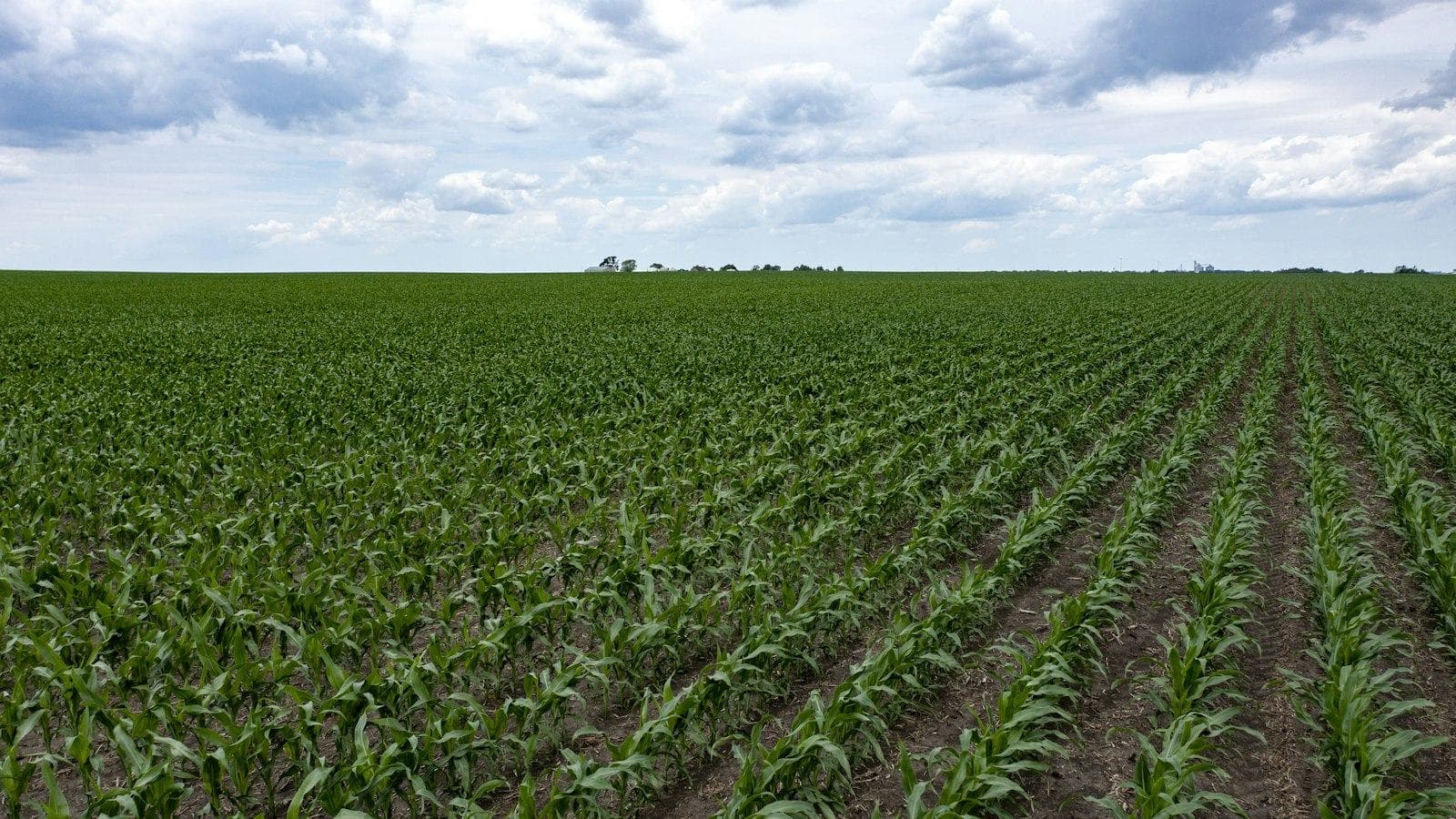
NDVI tells you how much green canopy is there. NDRE tells you how green that canopy is, which tracks chlorophyll and therefore nitrogen status, and it keeps working after NDVI saturates in a dense crop. GNDVI sits between the two. Use NDVI early in the season, NDRE from canopy closure onward, and GNDVI as a 10 m chlorophyll proxy.
This article covers the Sentinel-2 band math for each index, a growth-stage table, why NDVI saturates, cloud masking with the SCL band, and a short Python script that computes all three.
NDVI vs NDRE vs GNDVI: what is the difference?
All three are normalised differences between near-infrared (NIR) reflectance and one other band. Leaves reflect strongly in the NIR and absorb visible light through chlorophyll. The choice of absorbing band decides what each index is sensitive to.
| Index | Formula | Absorbing band | Responds most to | Weak point |
|---|---|---|---|---|
| NDVI | (NIR − Red) / (NIR + Red) | Red, ~665 nm | Green cover, biomass at low to moderate density | Saturates in dense canopies |
| NDRE | (NIR − RedEdge) / (NIR + RedEdge) | Red edge, ~705 nm | Canopy chlorophyll, nitrogen status | Noisier at low cover, 20 m on Sentinel-2 |
| GNDVI | (NIR − Green) / (NIR + Green) | Green, ~560 nm | Chlorophyll concentration | Less specific than NDRE, affected by soil brightness |
Red light is absorbed almost completely by chlorophyll, so red reflectance hits a floor quickly. Red-edge and green light are absorbed less strongly, so their reflectance keeps falling as chlorophyll rises. That is the whole story behind NDVI vs NDRE. GNDVI was proposed by Gitelson, Kaufman and Merzlyak (1996) precisely because the green band stays sensitive to chlorophyll over a wider range than red.
What are the Sentinel-2 band formulas for NDVI, NDRE and GNDVI?
Sentinel-2's MultiSpectral Instrument has three red-edge bands, which is the main reason it is the default free sensor for crop nitrogen work. The bands these indices use, from ESA's Sentinel-2 mission page on SentiWiki:
| Band | Role | Central wavelength S2A / S2B / S2C (nm) | Bandwidth (nm) | Native resolution |
|---|---|---|---|---|
| B3 | Green | 559.9 / 559.0 / 560.6 | 35 | 10 m |
| B4 | Red | 664.6 / 664.9 / 666.5 | 31 | 10 m |
| B5 | Red edge 1 | 704.1 / 703.8 / 707.1 | 14 to 16 | 20 m |
| B8 | NIR (broad) | 832.8 / 832.9 / 834.6 | 114 to 118 | 10 m |
| B8A | NIR (narrow) | 864.7 / 864.0 / 865.6 | 20 to 21 | 20 m |
The formulas on Sentinel-2 L2A surface reflectance:
NDVI   = (B8 - B4)  / (B8 + B4)      10 m native
GNDVI  = (B8 - B3)  / (B8 + B3)      10 m native
NDRE   = (B8A - B5) / (B8A + B5)     20 m native (recommended)
NDRE10 = (B8 - B5)  / (B8 + B5)      10 m output, B5 upsampled from 20 m
CIre   = (B8A / B5) - 1              20 m, red-edge chlorophyll index
The 20 m red-edge problem
B5 is a 20 m band. If you pair it with the 10 m B8 to get a "10 m NDRE", you have to upsample B5 first, and every 20 m B5 pixel becomes four identical 10 m pixels (or a smoothed version of them with bilinear resampling). The NIR numerator varies at 10 m, the red-edge term varies at 20 m, and the output looks sharper than the information it contains.
There is a second, less obvious issue. B8 is about 115 nm wide and B8A about 20 nm, so the two NIR bands see slightly different parts of the spectrum. NDRE values from B8/B5 and B8A/B5 are not interchangeable. Pick one definition per project and keep it for the whole time series.
My default is B8A/B5 at 20 m for anything that feeds a nitrogen decision, because both bands are native 20 m and closely matched in bandwidth. A 20 m pixel is 0.04 ha, so a 16 ha (40-acre) field still holds roughly 300 interior pixels. If you need 10 m output for display, compute at 20 m and resample the finished index, rather than resampling the input band and pretending the result is 10 m.
Convert L2A digital numbers to reflectance first
Since processing baseline 04.00, introduced on 25 January 2022, Sentinel-2 L2A products store reflectance with an additive offset. As ESA's announcement on the STEP forum explains, the conversion is:
reflectance = (DN + BOA_ADD_OFFSET) / BOA_QUANTIFICATION_VALUE
            = (DN - 1000) / 10000        for baseline 04.00 and later
DN = 0 is no data
Older products have no offset, and reprocessed archives can carry a newer baseline than their acquisition date suggests, so read the offset from each product's MTD_MSIL2A.xml rather than hard-coding it.
Here is what skipping it does. A crop pixel with true red reflectance 0.05 and NIR 0.35 has NDVI = 0.30 / 0.40 = 0.75. Its stored DNs are 1500 and 4500. Compute NDVI on those raw values (or on DN / 10000) and you get (4500 − 1500) / (4500 + 1500) = 0.50. The offset does not cancel in a normalised difference, and the error is largest for the dark red and red-edge bands.
Which index should I use at each growth stage?
The best index depends on the question and on how closed the canopy is. The nitrogen timing follows extension sensing windows.
| Stage | Main question | Best index | Why |
|---|---|---|---|
| Emergence to early vegetative (corn before about V6, wheat tillering, canola seedling) | Is the stand even? Where are the gaps? | NDVI | Soil is still visible, cover is the main signal, and NDVI has the most dynamic range at low cover |
| Nitrogen decision window (corn V6 to V10 per Oklahoma State Extension, later in Nebraska's Project SENSE; winter wheat after spring green-up and before hollow stem; winter canola just before bolting) | Is the crop short of nitrogen relative to a well-fed reference? | NDRE, with GNDVI as a 10 m cross-check | Canopy is filling in, NDVI is starting to compress, chlorophyll differences are what you care about |
| Closed canopy (corn around tasselling and grain fill, canola flowering) | Which zones are still stressed? | NDRE or CIre | NDVI is saturated, red-edge indices still separate zones |
| Senescence | Is the crop drying down evenly? | NDVI | Large, fast drop in green cover is exactly what NDVI measures well |
Canola flowering is a special case. Yellow petals change visible reflectance across the whole field, so any index that includes a visible band shifts during bloom for reasons unrelated to nitrogen. Compare flowering-period images only with other flowering-period images.
Why does NDVI saturate in a dense canopy?
NDVI saturation is arithmetic, not a sensor fault. In a closed canopy, red reflectance is already close to zero, so NDVI is close to its ceiling and can only change through NIR. The sensitivity of a normalised difference to NIR is:
d(NDVI)/d(NIR) = 2 * Red / (NIR + Red)^2
Take illustrative closed-canopy reflectances: red 0.03, red edge 0.12, NIR 0.45. Increase NIR by 0.10, roughly what extra leaf area might add:
| Index | Before | After NIR +0.10 | Change |
|---|---|---|---|
| NDVI (red 0.03) | 0.875 | 0.897 | +0.022 |
| GNDVI (green 0.06) | 0.765 | 0.803 | +0.039 |
| NDRE (red edge 0.12) | 0.579 | 0.642 | +0.063 |
The same change in the canopy moves NDRE about three times as far as NDVI, because the red-edge denominator is larger and the index sits far below its ceiling. On a map with a 0 to 1 colour ramp, that NDVI change is invisible.
Field data agree. In 24 field-years of maize and soybean data from eastern Nebraska, Nguy-Robertson et al. (2012, Agronomy Journal) found normalised difference indices such as NDVI were most sensitive to green leaf area index below about 2 m²/m², while ratio indices, including the chlorophyll indices, were most sensitive above it. For red-edge sensors, the combination of red-edge NDVI and the red-edge chlorophyll index estimated green LAI in both crops without re-calibration.
One practical caveat: NDRE is also a normalised difference, so it saturates too, just later. If you work in very dense corn, compute CIre = B8A / B5 − 1 alongside it. CIre has no ceiling and stays closer to linear at high chlorophyll content.
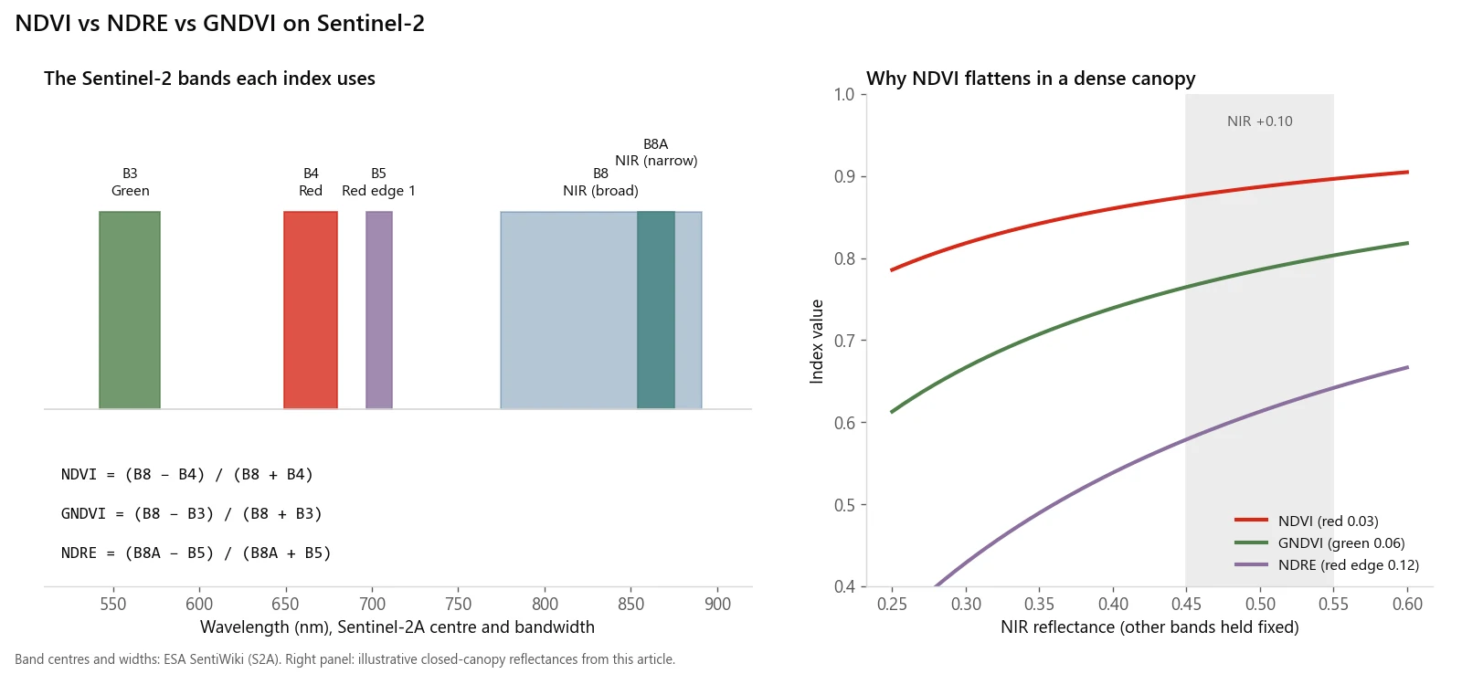
Which bands each index uses, and why NDVI stops responding in a dense canopy while NDRE keeps moving.
How do I mask clouds and shadows with the SCL band?
Every Sentinel-2 L2A product includes a 20 m Scene Classification Layer (SCL). The classes, from ESA's L2A processing documentation:
| SCL value | Class | Keep for crop indices? |
|---|---|---|
| 0 | No data | No |
| 1 | Saturated or defective | No |
| 2 | Cast shadows | Usually no; rare on flat cropland |
| 3 | Cloud shadows | No |
| 4 | Vegetation | Yes |
| 5 | Not vegetated | Yes (bare soil is a valid reading early in the season) |
| 6 | Water | Yes, but expect negative NDVI |
| 7 | Unclassified | Yes, with caution |
| 8 | Cloud, medium probability | No |
| 9 | Cloud, high probability | No |
| 10 | Thin cirrus | No |
| 11 | Snow or ice | No |
Three things the class table will not tell you:
- SCL under-detects cloud edges and thin haze. The pixels just outside a cloud are brighter in the visible bands than clear ground, which pushes NDVI down. Buffer the cloud and shadow mask by 100 m or so before computing field statistics.
- Never mask class 5 in-season. Bare soil between rows early in the season is exactly the signal NDVI is measuring. Masking it inflates the field mean.
- Set a minimum clear fraction per field. A field mean built from the 15% of pixels that dodged a cloud is not a field mean. A sensible default is to drop any field-date where less than about 80% of interior pixels are clear, and to report the clear fraction alongside every number.
SCL is 20 m, so upsample it to 10 m with nearest-neighbour resampling. Bilinear resampling averages class codes and invents classes that do not exist, for example averaging cloud shadow (3) and cloud (9) into water (6).
Python: compute NDVI, NDRE and GNDVI from a Sentinel-2 L2A tile
This script reads one unzipped L2A .SAFE product, applies the offset, masks clouds and shadows, and computes all three indices at their honest resolutions. It needs only rasterio and numpy.
import glob
import re

import numpy as np
import rasterio
from rasterio.enums import Resampling

SAFE = "path/to/S2X_MSIL2A_....SAFE"  # an unzipped L2A product

def band_path(res, name):
    return glob.glob(f"{SAFE}/GRANULE/*/IMG_DATA/R{res}m/*_{name}_{res}m.jp2")[0]

# Offset is -1000 from processing baseline 04.00 on, absent before it.
mtd = open(f"{SAFE}/MTD_MSIL2A.xml").read()
m = re.search(r"<BOA_ADD_OFFSET[^>]*>(-?\d+)<", mtd)
OFFSET = int(m.group(1)) if m else 0
QUANT = int(re.search(r"<BOA_QUANTIFICATION_VALUE[^>]*>(\d+)<", mtd).group(1))

def read(path, shape=None):
    with rasterio.open(path) as src:
        return src.read(1, out_shape=shape, resampling=Resampling.nearest)

def reflectance(dn):
    r = (dn.astype("float32") + OFFSET) / QUANT
    r[dn == 0] = np.nan  # DN 0 is no data
    return r

# 10 m bands for NDVI and GNDVI
b3, b4, b8 = (reflectance(read(band_path(10, b))) for b in ("B03", "B04", "B08"))
# 20 m bands for NDRE, kept at native resolution
b5, b8a = (reflectance(read(band_path(20, b))) for b in ("B05", "B8A"))

scl20 = read(band_path(20, "SCL"))
scl10 = read(band_path(20, "SCL"), shape=b4.shape)  # nearest: never average class codes

BAD = [0, 1, 3, 8, 9, 10, 11]  # no data, defective, cloud shadow, clouds, cirrus, snow

def norm_diff(a, b, scl):
    with np.errstate(divide="ignore", invalid="ignore"):
        out = (a - b) / (a + b)
    out[np.isin(scl, BAD)] = np.nan
    return out

ndvi = norm_diff(b8, b4, scl10)
gndvi = norm_diff(b8, b3, scl10)
ndre = norm_diff(b8a, b5, scl20)  # 20 m, both bands native

for name, arr in (("NDVI", ndvi), ("GNDVI", gndvi), ("NDRE", ndre)):
    print(f"{name}: median {np.nanmedian(arr):.3f}, clear {np.isfinite(arr).mean():.0%}")
A full tile is 10,980 × 10,980 pixels at 10 m, so this needs a few gigabytes of RAM. For a single farm, pass a window= to src.read built from the field boundary. To save results, copy the profile of the matching source band and set dtype="float32" and nodata=np.nan.
How does sen2auto compute these indices at provincial scale?
The script above handles one tile on one date. A region, a crop insurer's book or a provincial program spans dozens of roughly 110 km MGRS tiles, often across a UTM zone boundary, and no single date is cloud-free everywhere.
I built sen2auto for that case. It downloads Sentinel-2 L2A scenes from the Copernicus Data Space Ecosystem, mosaics them onto one grid, and computes NDVI, NDRE, GNDVI and several other indices, including CIre. The design choices map directly onto the pitfalls above:
- Offset per product. The BOA offset is read from each product's metadata, not assumed, so mixed-baseline archives come out consistent.
- One target grid across UTM zones. Every scene is warped onto a single grid with a snapped origin, so tiles from adjacent zones line up pixel for pixel.
- Cloud-aware compositing. Where scenes overlap, each pixel comes from the best-ranked clear observation (ranked on cloud cover, closeness to the target date and orbit consistency), with the SCL mask buffered by 100 m. It deliberately does not use brightest-pixel compositing, which favours cloud at every seam.
- Least-squares tile levelling. One gain and offset per scene and band is solved from clear-land overlaps to remove seams between dates. This is relative normalisation: it makes the mosaic consistent, not more absolutely accurate.
- No fabricated gaps. Pixels with no clear observation stay as no data instead of being filled with averages.
How do US and Canadian growers use these indices for nitrogen?
The in-season nitrogen work in North American extension programs is mostly done with proximal sensors (on the applicator or handheld), but the logic transfers directly to satellite indices.
Corn, Nebraska. The University of Nebraska–Lincoln's Project SENSE put crop canopy sensors on a high-clearance applicator so that sensing and in-season nitrogen application happen in one pass (CropWatch). The on-farm reports show the sensors captured NDRE. Two 2017 trials show how varied the results are:
- In York County, sensing at V16 led to 216 lb N/acre in total against the grower's 210, and yields of 248 and 247 bu/acre, with no significant difference (UNL report).
- In Nance County, the applicator sensors at V13 used 43 lb N/acre less than the grower and yielded significantly less (229 against 238 bu/acre). A drone NDRE map of the same field, flown three days earlier, called for 100 lb N/acre in-season against the applicator's 60, and the report notes it is not clear why the two NDRE sources disagreed so much (UNL report).
The honest takeaway: NDRE carries real nitrogen information, but the rate it produces depends on the sensor and its calibration. Two NDRE maps of the same field are not the same measurement.
Winter wheat, Oklahoma. Oklahoma State's approach compares NDVI on a nitrogen-rich reference strip with the adjacent field, using a GreenSeeker sensor, and feeds both readings to a free sensor-based nitrogen rate calculator. Wheat is sensed after spring green-up and before hollow stem, when the canopy is still open enough for NDVI to work.
Canola, Prairies. A project summarised on the Canola Council of Canada's research hub, run at Indian Head (SK), Brandon (MB) and Edmonton (AB) tested NDVI optical sensors for variable-rate in-crop nitrogen in canola and concluded the sensor shows promise for variable nitrogen application.
The transferable piece is the reference strip. A ratio such as NDRE(field) / NDRE(well-fed strip) cancels much of the date-to-date variation from sun angle, haze and crop stage, which is why it works across sensors when raw values do not. For satellite use, the strip has to be wide enough to contain whole pixels. A strip at least 40 m wide always contains at least one complete 20 m pixel across its width, whatever the grid alignment. A narrower strip may contain none.
Index values also differ by crop, so stratify before comparing. In the US, the USDA NASS Cropland Data Layer moved to 10 m resolution with the 2024 edition. In Canada, the AAFC Annual Crop Inventory is a 30 m national crop map. Either gives you a crop mask, so you are not averaging canola into wheat.
When is a vegetation index the wrong tool?
- When you need a diagnosis, not a symptom. Any stress that reduces chlorophyll lowers NDRE and GNDVI: nitrogen, but also drought, disease, waterlogging and other nutrient deficiencies. An index tells you where to look. Tissue tests, soil tests and a field walk tell you why.
- When you compare absolute values across sensors. Sentinel-2, PlanetScope, Landsat, drone cameras and GreenSeeker all give different NDVI for the same crop. Calibrate within a sensor, or use ratios against a reference.
- When fields are small or narrow. A 20 m NDRE pixel is wider than many research plots and shelterbelt-edged strips. See the field-size rule of thumb in Sentinel-2 vs Landsat vs Planet for crop monitoring.
- When the decision cannot wait for clear sky. If a nitrogen window closes during a wet week, on-machine sensors or a planned rate will beat waiting for an image.
If you need an index pipeline, a field-level monitoring report or a regional Sentinel-2 mosaic scoped or built, email me at mahad.imran29@gmail.com.