To estimate population for a custom area, such as a trade area, a 2 km buffer or a new service zone, start from the smallest source zones you can get, then use area weighting or, better, dasymetric mapping to move their counts into your area. In a test of 2,400 random circles in Calgary and Islamabad, zone size mattered far more than method: a 2 km circle built from 5 km² zones had a median error of 5.8%, while the same circle built from 36 km² zones was off by a median 22%.
This is one of the most common jobs in applied GIS, and one of the least discussed. Population is published for census tracts, wards, union councils or tehsils. The question a client asks is about a different shape: a drive-time trade area, a catchment around a clinic, a franchise territory. Moving the numbers from one set of zones to the other is called areal interpolation, and the way you do it decides how wrong the answer is.
What is areal interpolation?
Areal interpolation transfers a count or a rate from source zones (the units the data comes in) to target zones (the units you need). The three approaches you will meet in practice are:
| Method | What it assumes | When it is fine |
|---|---|---|
| Centroid rule | A source zone belongs entirely to the target if its centre falls inside | Source zones are tiny compared with the target |
| Area weighting | People are spread evenly across each source zone | Source zones are small, or population really is even |
| Dasymetric mapping | People live only on certain land, given by an ancillary layer | You have a reliable layer of where people can live |
Area weighting was set out for GIS by Goodchild and Lam in 1980, in a paper titled Areal interpolation: a variant of the traditional spatial problem. If a source zone of 20,000 people is 30% inside your target by area, the target gets 6,000 of them. Dasymetric mapping, which has a long cartographic history and was formalised for GIS work by Mennis (2003), first removes land where nobody lives (water, parks, industrial land, farmland) and then spreads people only across what is left.
There is a fourth family, pycnophylactic and statistical methods such as Tobler's smooth interpolation, which assume density changes smoothly across zone edges. They are rarely worth the effort for business questions, and they are not tested here.
How did I test the methods?
I needed a case where the true answer is known, so I worked backwards from fine data to coarse data:
- Reference population: Kontur Population on H3 resolution 8 hexagons, about 0.74 km² each, for Calgary (1,205 hexagons, 1.46 million people) and Islamabad Capital Territory (1,164 hexagons, 2.59 million people). These are the same layers behind the Site Selection Showdown game. They are modelled, so I treat them as the reference, not as the truth on the ground.
- Source zones: I rolled the hexagons up to their H3 parents at resolution 7 (about 5.2 km², similar to an urban census tract) and resolution 6 (about 36 km², closer to a ward, a tehsil or a large municipal district). Calgary has 215 and 41 of these, Islamabad 200 and 39.
- Targets: 400 circles each of 1 km, 2 km and 3 km radius per city, 2,400 in total. Each centre was drawn in proportion to population, with a few hundred metres of random jitter, so the circles land where real analyses land: in places where people live.
- Ancillary layer for dasymetric mapping: the OpenStreetMap land-use flag from the same dataset, which marks hexagons that are mostly park, water, forest or airfield, or that have no drivable road. That is the kind of mask a planner can build in an afternoon.
- Error: the estimate from each method minus the reference count in the circle, as a percentage.
The H3 resolution guide has the full table of cell sizes if you want to repeat this at other scales.
What did the test show?
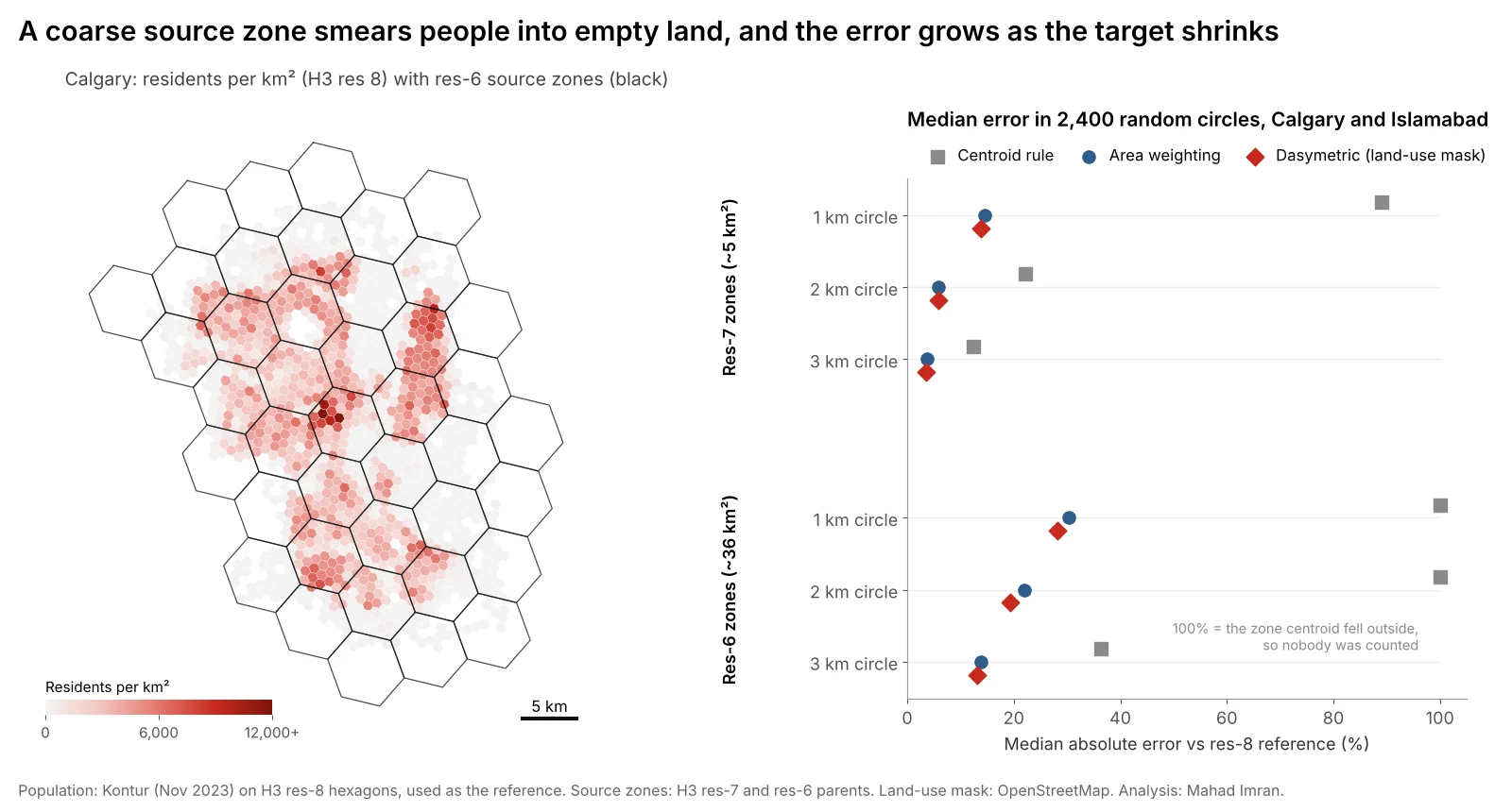
Median absolute error across 2,400 circles in Calgary and Islamabad. Square markers at 100% mean no zone centroid fell inside the circle, so the centroid rule counted nobody.
| Source zones | Circle radius | Centroid rule | Area weighting | Dasymetric |
|---|---|---|---|---|
| ~5 km² (res 7) | 1 km | 89% | 14.6% | 13.8% |
| ~5 km² (res 7) | 2 km | 22% | 5.8% | 5.9% |
| ~5 km² (res 7) | 3 km | 12% | 3.7% | 3.5% |
| ~36 km² (res 6) | 1 km | 100% | 30% | 28% |
| ~36 km² (res 6) | 2 km | 100% | 22% | 19% |
| ~36 km² (res 6) | 3 km | 36% | 14% | 13% |
Median absolute error. The share of circles off by more than 20% tells the same story more bluntly:
| Source zones | Circle radius | Centroid rule | Area weighting | Dasymetric |
|---|---|---|---|---|
| ~5 km² | 2 km | 55% | 3% | 4% |
| ~36 km² | 2 km | 98% | 56% | 49% |
Four findings stand out.
1. Source zone size matters more than the method
Moving from 36 km² zones to 5 km² zones cut the median error for a 2 km circle from 22% to 5.8% with plain area weighting. No choice of method came close to that. If you can get block-level, dissemination-area or tract-level data instead of a district total, do that before anything else.
A useful rule from these numbers: area weighting is comfortable when the target is at least two to three times wider than the source zones. A 2 km circle covers about 12.6 km², roughly two and a half res-7 zones, and errors were small. The same circle against 36 km² zones covers about a third of one zone, and errors were large.
2. The centroid rule is worse than it looks
Counting zones whose centre falls inside the buffer is the default in many quick analyses because it needs no overlay. It produced a median error of 22% for a 2 km circle even from small zones, and with 36 km² zones it found no zone at all in 98% of 2 km circles. When it does catch a zone, it counts every resident of it, so a 3 km circle from res-6 zones was off by a median 36% in either direction.
3. Area weighting is biased low where people live
Area weighting does not just add noise. Because analysts draw buffers around places where people are, and the method spreads each zone's population evenly into its empty parts, it underestimates dense places. From res-6 zones, the median 2 km circle in Calgary came out 22% low, and in Islamabad 12.5% low. A retail model built this way will systematically under-call urban sites and over-call fringe ones.
4. Dasymetric mapping helps, but only as much as the mask removes
The land-use mask lowered errors everywhere, but by a few points at most: from 22.0% to 19.4% at 2 km from res-6 zones. The reason is simple. In Calgary, 92% of the land passed the mask, so it barely changed where people were placed. In Islamabad 78% passed, and the gain there was bigger (18.9% to 16.5% in the same test).
I also tried weighting by road connectivity, using the number of candidate sites that can reach each hexagon within 12 minutes as a stand-in for road density. It cut Islamabad's res-6 error at 2 km from 18.9% to 14.0% but did nothing for Calgary. The lesson is that an ancillary layer must separate empty land from settled land inside the source zones you have. Building footprints do that well. A coarse land-cover class usually does not.
Which method should you use?
| Situation | Recommended approach |
|---|---|
| You have small zones (blocks, dissemination areas, tracts) and a large target | Area weighting is enough |
| You only have large zones and a small target | Dasymetric with building footprints or a gridded population layer |
| You have a gridded population layer for the area | Skip interpolation and sum the grid directly |
| Zones have large lakes, parks or industrial land | At least mask those out before weighting |
| Quick screening of many buffers | Area weighting, never the centroid rule |
A gridded population product, such as WorldPop, GHSL, Meta's high-resolution maps or Kontur, is itself the output of a dasymetric model built with satellite-detected buildings. For most target areas, summing that grid is the quickest route to a defensible number. The trade-offs between those grids are in WorldPop vs LandScan vs GHSL vs Kontur. If you need the official census total, rescale the grid so it matches the census count of each source zone, which keeps the official totals and borrows the grid's sense of where people live inside each zone.
How do you do areal interpolation in Python?
PySAL's tobler package covers both methods. Area weighting from census tracts to a set of trade areas looks like this:
import geopandas as gpd
from tobler.area_weighted import area_interpolate

tracts = gpd.read_file("tracts.gpkg").to_crs(32611)       # UTM 11N for Calgary
trade_areas = gpd.read_file("trade_areas.gpkg").to_crs(32611)

est = area_interpolate(
    source_df=tracts,
    target_df=trade_areas,
    extensive_variables=["population", "households"],  # counts: split by area
    intensive_variables=["median_income"],               # rates: area-weighted average
)
trade_areas[["population", "households"]] = est[["population", "households"]]
Two details trip people up:
- Project first. Area shares must be computed in an equal-area or local projected CRS, never in degrees or Web Mercator. Web Mercator inflates areas by the square of 1/cos(latitude), which in Calgary is about 2.5 times. Why your web map gets distance and area wrong has the details.
- Counts and rates are different. Population and households are extensive and get split by area. Median income or a literacy rate are intensive and should be averaged, ideally weighted by population, never summed.
For a dasymetric version, tobler's masked_area_interpolate takes a land-cover raster and the pixel classes to keep. If you have building footprints instead, the manual approach is short: intersect footprints with source zones, give each footprint a share of its zone's population by floor area, then sum footprints inside each target.
# Dasymetric with building footprints, manual version
b = gpd.overlay(buildings, tracts[["tract_id", "population", "geometry"]])
b["w"] = b.area                                     # or area * floors
b["pop"] = b["population"] * b["w"] / b.groupby("tract_id")["w"].transform("sum")
est = gpd.sjoin(b.set_geometry(b.centroid), trade_areas).groupby("index_right")["pop"].sum()
What are the limits of this test?
- The reference is a model. Kontur hexagons are themselves dasymetric estimates. Real census blocks would show more local variation, which would make every method look worse, the coarse ones most of all.
- Circles are friendly targets. Drive-time polygons and irregular territories have more edge per unit area, which usually adds error.
- One kind of mask. I tested a land-use mask available everywhere OpenStreetMap is mapped. Building footprints from Microsoft, Google or OpenStreetMap would likely do better, and I would expect the gain to be largest in Islamabad, where large green belts sit inside the sector grid.
- Two cities. A sprawling suburban city and a planned capital with forested hills. Dense old cores, such as inner Lahore or Karachi, would stress the methods differently.
What should you take from this?
Before you argue about methods, check how big your source zones are compared with the area you are estimating. If the zones are larger than the target, no clever weighting will rescue the number, and you should find finer data or a gridded population layer. If they are small, plain area weighting in a projected CRS is accurate to a few percent. Avoid the centroid rule for anything but a quick look.
If you need population, households or customers estimated for trade areas, service zones or territories, email me at mahad.imran29@gmail.com.