The fastest point-in-polygon method in Python depends on the shape of your polygons. For a few large polygons, prepared geometries with shapely.contains_xy assigned 10 million points in 2.9 to 3.6 seconds. For thousands of small polygons, geopandas.sjoin or an STRtree took 13 to 18 seconds, and an H3 lookup 9.6 seconds. The biggest trap was building the spatial index on the wrong side: on detailed district boundaries it turned a 13.5-second join into a 2-minute one.
Assigning points to polygons is one of the most common jobs in spatial data work: geocoded customers to sales territories, GPS pings to zones, incidents to fire districts, survey households to union councils. At thousands of points any method works. At millions, the method you pick decides whether the job takes seconds or a coffee break. I benchmarked six approaches on three polygon layers to find out which to use when.
How was the benchmark set up?
Polygon layers, chosen to cover the cases people actually meet:
| Layer | Polygons | Vertices in total | Typical use |
|---|---|---|---|
| Calgary H3 hexagons (resolution 8) | 1,205 | 8,435 | Many small zones: grids, neighbourhoods, postcodes |
| Punjab districts, simplified | 36 | 5,046 | A few large zones, web-map quality boundaries |
| Punjab districts, detailed | 36 | 101,415 | A few large zones, survey-grade boundaries |
The detailed Punjab layer is the simplified one with extra vertices inserted every 0.0015° (about 150 m), so the shapes are identical and only the vertex count changes. That isolates the effect of boundary detail.
Points: 100,000, 1 million and 10 million per layer, in WGS84 longitude and latitude. Calgary points were drawn in proportion to population from the Kontur hexagons with a little random scatter. Punjab points were uniform over the province's bounding box, so a share of them fall outside every district, as real data often does.
Machine and software: a single Python process on a 4-vCPU cloud VM, Python 3.13, GeoPandas 1.2, Shapely 2.2 and h3-py 4.5. Times include building point geometries where a method needs them. Every method was checked against the STRtree result, and all exact methods agreed on 100% of points.
The six methods:
- Python loop: for each point, test each polygon with
polygon.contains(point)until one matches. - STRtree on polygons: build
shapely.STRtreeon the polygons and query it with all points,predicate="within". - STRtree on points: build the tree on the points and query it with the polygons,
predicate="contains". - GeoPandas sjoin:
gpd.sjoin(points, polygons, predicate="within"). - Prepared polygons: for each polygon,
shapely.prepare, keep points inside its bounding box, then test them withshapely.contains_xy. - H3 lookup: convert each point to an H3 cell with
h3.latlng_to_celland look the cell up in a dictionary built from the polygons.
What were the results?
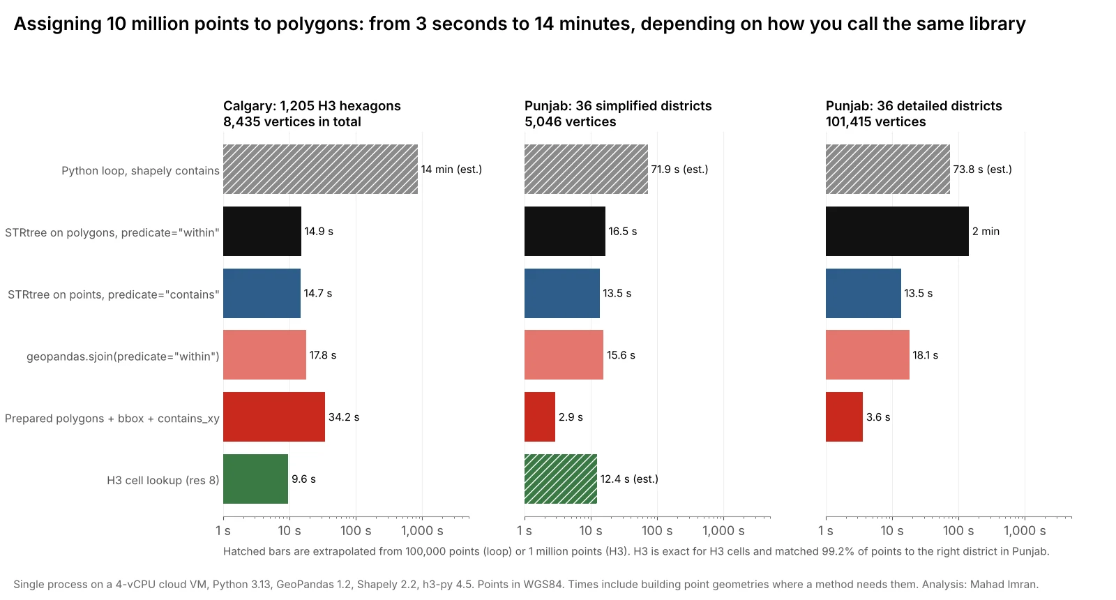
Seconds to assign 10 million points:
| Method | Calgary hexagons | Punjab, simplified | Punjab, detailed |
|---|---|---|---|
| Python loop | ~853 (est.) | ~72 (est.) | ~74 (est.) |
STRtree on polygons, within | 14.9 | 16.5 | 142.6 |
STRtree on points, contains | 14.7 | 13.5 | 13.5 |
geopandas.sjoin | 17.8 | 15.6 | 18.1 |
Prepared + bbox + contains_xy | 34.2 | 2.9 | 3.6 |
| H3 lookup (resolution 8) | 9.6 | ~12 (est.), approximate | n/a |
Loop times are extrapolated from 100,000 points and the Punjab H3 time from 1 million, because all methods scaled close to linearly. At 1 million points:
| Method | Calgary hexagons | Punjab, simplified | Punjab, detailed |
|---|---|---|---|
| STRtree on polygons | 1.49 | 1.65 | 14.25 |
| STRtree on points | 1.09 | 1.02 | 1.06 |
geopandas.sjoin | 1.45 | 1.25 | 1.45 |
Prepared + bbox + contains_xy | 2.18 | 0.22 | 0.30 |
| H3 lookup | 0.92 | 1.24 (res 8) | n/a |
What do the results mean?
1. Never loop over points in Python
The loop gave the right answer and was the slowest by far: an estimated 14 minutes for 10 million points against 1,205 hexagons, around 90 times slower than an H3 lookup and 50 times slower than sjoin. Every loop iteration creates a Python object and calls into GEOS once. Vectorised Shapely 2 functions do the same work in C, over whole arrays.
2. A few big polygons: prepare them and filter by bounding box
With 36 districts, the prepared approach was 5 times faster than sjoin: 2.9 seconds against 15.6. It loops over polygons, not points, so there are only 36 Python iterations. For each one, a cheap NumPy comparison throws out points outside the district's bounding box, and contains_xy tests the rest without ever building point objects. Preparing the polygon builds an internal index of its edges, which is why adding 20 times more vertices only moved the time from 2.9 to 3.6 seconds.
import numpy as np
import shapely

def assign_points(x, y, polygons):
    """Index of the polygon containing each point, or -1. x, y are NumPy arrays."""
    out = np.full(len(x), -1)
    shapely.prepare(polygons)
    for k, poly in enumerate(polygons):
        xmin, ymin, xmax, ymax = shapely.bounds(poly)
        idx = np.flatnonzero((x >= xmin) & (x <= xmax) & (y >= ymin) & (y <= ymax))
        inside = shapely.contains_xy(poly, x[idx], y[idx])
        out[idx[inside]] = k
    return out

district = assign_points(df.lon.values, df.lat.values, districts.geometry.values)
The same approach was the slowest exact method on Calgary's 1,205 hexagons, at 34 seconds, because each of the 1,205 iterations scans all 10 million coordinates for the bounding-box filter. It is the right tool for tens of polygons, not thousands.
3. Many small polygons: sjoin or an STRtree, built the right way round
With 1,205 hexagons, sjoin and both STRtree variants landed between 14.7 and 17.8 seconds. Here the spatial index does the real work, narrowing each point to one or two candidate hexagons. sjoin is the most convenient, because it keeps attributes and returns a GeoDataFrame:
import geopandas as gpd

pts = gpd.GeoDataFrame(df, geometry=gpd.points_from_xy(df.lon, df.lat), crs=4326)
joined = gpd.sjoin(pts, zones[["zone_id", "geometry"]], how="left", predicate="within")
Two details matter. Build points with points_from_xy, never by applying Point() row by row. And make sure both layers share the same CRS before joining, which GeoPandas warns about but does not enforce.
4. The side you index matters on detailed boundaries
This was the surprise. On the detailed districts, an STRtree built on the polygons and queried with 10 million points took 142.6 seconds. Building the tree on the points and querying with 36 polygons took 13.5 seconds, for exactly the same assignments.
Shapely tests the predicate between each query geometry and its candidate tree geometries. With the tree on polygons, every one of the 10 million point queries runs a point-in-polygon test against a raw polygon of up to several thousand vertices. With the tree on points, there are only 36 query geometries, and each detailed polygon's cost is paid once per polygon rather than once per point. sjoin was not slowed by the detailed boundaries either, at 18.1 seconds, so the convenient option also avoided the trap.
import numpy as np
import shapely

points = shapely.points(x, y)
tree = shapely.STRtree(points)                       # index the many simple geometries
poly_idx, pt_idx = tree.query(polygons, predicate="contains")
zone = np.full(len(points), -1)
zone[pt_idx] = poly_idx
The general rule: index the many simple geometries, and query with the few complex ones.
5. H3 is the fastest when your zones are H3 cells
When the polygons are H3 cells, converting each point to its cell and looking it up in a dictionary is not an approximation. It is the definition. It took 9.6 seconds for 10 million points, the fastest result on that layer, even though h3-py was called one point at a time from Python. It agreed with the geometric join on 99.97% of points. The remaining 0.03% is most likely down to the hexagon outlines in my file, which are rounded to 5 decimal places and so differ by up to about a metre from H3's own cell edges.
For other polygons, H3 gives an approximation. I filled each Punjab district with H3 cells and looked points up the same way:
| H3 resolution | Average cell area | Cells for Punjab | Points matched to the right district | Points left unassigned |
|---|---|---|---|---|
| 7 | 5.2 km² | 36,833 | 98.0% | 0.4% |
| 8 | 0.74 km² | 257,864 | 99.2% | 0.15% |
Errors sit along district borders, where a cell is assigned to whichever district holds its centre. For a heat map or a dashboard that is fine. For anything with money or legal weight attached, such as tax districts, insurance zones or NG911 emergency service boundaries, use an exact geometric test.
Which method should you use?
| Your situation | Use |
|---|---|
| Up to a few hundred thousand points, any polygons | geopandas.sjoin, for convenience |
| A few to a few dozen large polygons, millions of points | Prepared polygons + bounding-box filter + contains_xy |
| Hundreds to thousands of polygons, millions of points | sjoin, or an STRtree built on the points |
| Your zones are H3 cells | H3 cell lookup |
| Approximate counts for a dashboard, any zones | Pre-fill zones with H3 cells, then look up |
| Detailed boundaries and a raw STRtree | Build the tree on the points, not the polygons |
| Data that does not fit in memory | A spatial database such as PostGIS, or chunked processing |
How can you make it faster still?
- Use all your cores. Every method here ran on one core. Splitting the points into chunks and processing them with
concurrent.futuresordask-geopandasscales close to linearly for this kind of embarrassingly parallel task. - Keep data in columnar formats. Reading 10 million points from CSV can take longer than the join itself. GeoParquet loads much faster, as measured in the geospatial file format benchmark.
- Simplify boundaries when exact edges do not matter. A district outline with 100,000 vertices is rarely needed for a point join. Simplify with a tolerance smaller than your positional error, typically a few metres.
- Do the work in the database if the data lives there. PostGIS with a GiST index, or an embedded engine such as DuckDB with its spatial extension, avoids moving millions of rows into Python at all. I did not include those in this benchmark, which focuses on the Python libraries most analysts already use.
- Check your CRS before optimising. A join between layers in different coordinate systems can return no matches at all, very quickly. And if you are measuring distances or buffers around the points, read why Web Mercator gets distance and area wrong first.
What are the limits of this benchmark?
- One machine, one run per test. Absolute times will differ on your hardware. The ratios between methods were stable across the three point counts, which suggests they will carry over.
- Points in memory. Times exclude reading the points from disk.
- Synthetic points. Calgary points follow population and Punjab points are uniform. Heavily clustered data, such as GPS traces on a few roads, changes how much work the bounding-box filter saves.
- Polygons without holes or overlaps. Overlapping zones return several matches per point, which
sjoinhandles and my simpleassign_pointsfunction does not.
What should you take from this?
Start with geopandas.sjoin: it was never the fastest, but it was never the trap either, landing between 15.6 and 18.1 seconds on every layer. When you need more speed, match the method to your polygons. For a few large zones, prepare them and use contains_xy, which was 5 times faster here. For H3 zones, use H3 lookups. If you work with a raw STRtree, build it on the many simple geometries. And whatever you choose, keep the loop out of Python.
If you have a large geocoding, assignment or spatial join pipeline that needs to run faster or more reliably, email me at mahad.imran29@gmail.com.